Graphing Quadratic Functions:
Quadratic equations in standard form are represented as \(\begin{array}{l}ax^2~+~bx~+~c~=~0\end{array} \)
where \(\begin{array}{l}a~\neq~0\end{array} \)
and \(\begin{array}{l}a,b,c\end{array} \)
are real constants. The roots or solutions of this equation can be found out using factorization method, completing the square method, by using quadratic formula or by using graphs.
To plot any function \(\begin{array}{l}y~+~f(x)\end{array} \)
, values of are substituted in given function and corresponding values of are obtained, using these co-ordinates graph is plotted. The graph of a quadratic function is represented using a parabola. If \(\begin{array}{l}\alpha\end{array} \)
and \(\begin{array}{l}\beta\end{array} \)
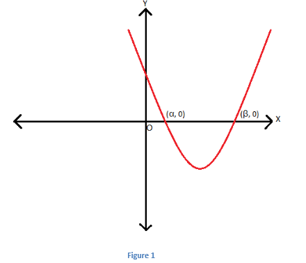
are real roots of a quadratic equation then, point of intersection of graph of the function with x -axis or the x – intercepts on graph represents its solution. Given figure represents a quadratic function with real roots \(\begin{array}{l}\alpha\end{array} \)
and \(\begin{array}{l}\beta\end{array} \)
.
The graph of a quadratic function is a parabola which can be represented in two forms:
- Standard Form:
\(\begin{array}{l}ax^2~+~bx~+~c\end{array} \)
- Vertex Form or
\(\begin{array}{l}(a~-~h~-~k)\end{array} \)
form: \(\begin{array}{l}f(x)~=~a(x~-~h)^2~+~k\end{array} \)
, where \(\begin{array}{l}(h,k)\end{array} \)
is vertex of parabola.
The graph opens upwards if \(\begin{array}{l}a > 0\end{array} \)
and downwards if \(\begin{array}{l}a < 0\end{array} \)
and depending upon value of a, the concavity of the graph or the rate of increase or decrease of function is affected. Simply, if a decreases, graph opens up and vice –versa. The change in value of alters the vertical position of graph and has no affect on its shape.
Vertex of a quadratic equation is its minimum or lowest point if the parabola is opening upwards or its highest or maximum point if it opens downwards.
On rearranging the standard form, vertex form is obtained by completing the square method.
On comparing both forms,
\(\begin{array}{l}h\end{array} \)
= \(\begin{array}{l}-\frac{b}{2a}\end{array} \)
\(\begin{array}{l}k\end{array} \)
= \(\begin{array}{l}f(h)\end{array} \)
When a quadratic function is represented in vertex form, following points are to be noted:
- If h > 0, graph shifts right by h units.
- If h < 0, graph shifts left by h units.
- If k > 0, graph shifts upwards by k units.
- If k < 0, graph shifts downwards by k units.
- (h, k) denotes the vertex of function.
For graphing a quadratic function, above steps are followed and further transformations are used.
Using Transformations to Graph Quadratic Functions:
-
i) Horizontal shifting by m units:
Consider the standard form of quadratic equation \(\begin{array}{l}ax^2~+~bx~+~c~=~0\end{array} \)
, having \(\begin{array}{l}\alpha\end{array} \)
and \(\begin{array}{l}\beta\end{array} \)
as roots.
Suppose instead of \(\begin{array}{l}\alpha\end{array} \)
and \(\begin{array}{l}\beta\end{array} \)
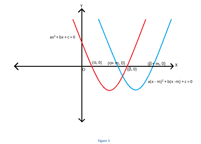
as roots of the quadratic equation, roots are given as \(\begin{array}{l}(\alpha~+~m)\end{array} \)
and \(\begin{array}{l}(\beta~+~m)\end{array} \)
. To plot such an equation, the original graph is shifted right by, as shown in figure given below. The equation representing this is given as:\(\begin{array}{l}a(x~-~m)^2~+~b(x~-~m)~+~c~=~0\end{array} \)
.
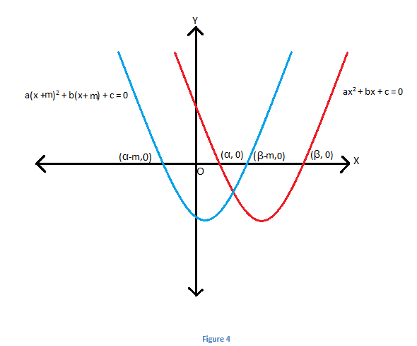
Similarly, if roots are \(\begin{array}{l}(\alpha~-~m)\end{array} \)
and \(\begin{array}{l}(\beta~-~m)\end{array} \)
instead of \(\begin{array}{l}\alpha\end{array} \)
and \(\begin{array}{l}\beta\end{array} \)
, then graph shifts left by \(\begin{array}{l}m\end{array} \)
units and the equation is given by: \(\begin{array}{l}a(x~+~m)^2~+~b(x~+~m)~+~c~=~0\end{array} \)
. This is shown as below:
-
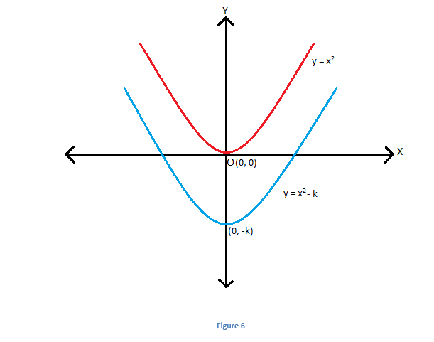
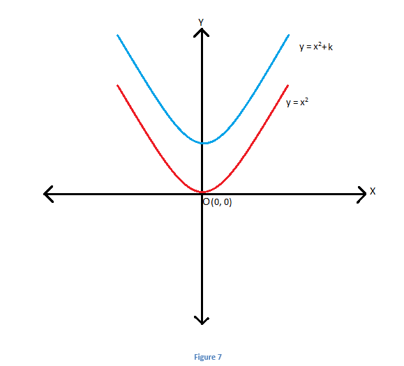
ii) Vertical shifting by k units:
Considering the vertex form i.e.,\(\begin{array}{l}y\end{array} \)
= \(\begin{array}{l}a(x~-~h)^2~+~k\end{array} \)
. To shift the graph vertically changes are made in the value of k. As already mentioned:
- If k > 0 , graph shifts upwards by k units.
- If k < 0 , graph shifts downwards by k units.
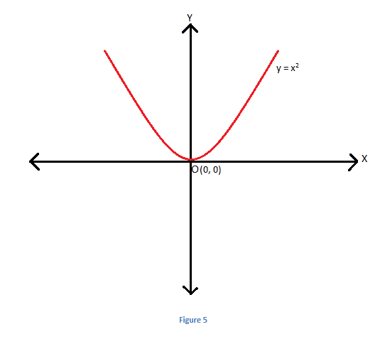
Let us first consider the graph of \(\begin{array}{l}y\end{array} \)
= \(\begin{array}{l}x^2\end{array} \)
. It represents a parabola with vertex at (0,0) as shown:
Let us go through an example for a better understanding.
Example: Find range of \(\begin{array}{l}x\end{array} \)
if \(\begin{array}{l}x^2~-~6x~+~5~\leq~0\end{array} \)
and \(\begin{array}{l}x^2~-~2x~\gt~0\end{array} \)
.
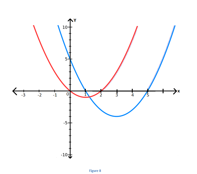
Solution: Let us try to graph the given equations to find out range of \(\begin{array}{l}x\end{array} \)
. As \(\begin{array}{l}a > 0\end{array} \)
for both inequalities therefore the graphs will be upward opening parabolas.
Let \(\begin{array}{l}x^2~-~6x~+~5~\leq~0\end{array} \)
………….(1) and \(\begin{array}{l}x^2~-~2x~\gt~0\end{array} \)
…….(2)
From equation (1),\(\begin{array}{l}(x~-~1)(x~-~5)~\leq~0\end{array} \)
. The blue parabola represents this inequality in fig. 8.
\(\begin{array}{l}\Rightarrow~1~\leq~x~\leq~5\end{array} \)
From equation (2), \(\begin{array}{l}(x~-~0)(x~-~2)~\gt~0\end{array} \)
.
\(\begin{array}{l}\Rightarrow~x~\lt~0\end{array} \)
or \(\begin{array}{l}x~\gt~2\end{array} \)
Thus, range of \(\begin{array}{l}x\end{array} \)
is: \(\begin{array}{l}2~\lt~x~\leq~5\end{array} \)
Thus graphing quadratic functions becomes easy using transformations.’

Comments