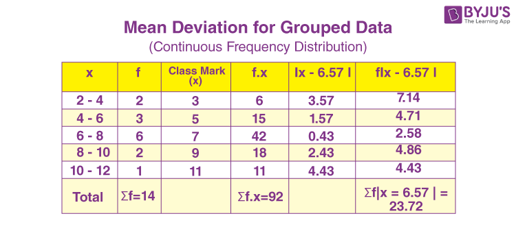
Data representation in a tabular or graphical form indicates the frequency (number of times an observation occurs within a particular interval) is known as a frequency distribution.
If the data is huge, for example, if we need to analyze the marks of 200 students, then the representation of such data in a random fashion is not very practical. So, we use the concept of ‘Grouping of Data’ based on class intervals. In the upcoming discussion, we will discuss how to calculate the mean deviation for the continuous frequency distribution of data.

Mean Deviation of Grouped Data
In frequency distribution of continuous type, the class intervals or groups are arranged so that there are no gaps between the classes and each class in the table has its respective frequency. The class intervals are chosen in such a way that they must be mutually exclusive and exhaustive.
To understand the concept of continuous frequency distribution, let us take the following example:
The following table represents the age group of employees working in a certain company.
| Age Group | Number of people |
| 15-25 | 25 |
| 25-35 | 54 |
| 35-45 | 34 |
| 45-55 | 20 |
This representation is continuous in nature, and the frequency is mentioned according to the class interval.
Steps to Calculate Mean Deviation of Continuous Frequency Distribution
To calculate the mean deviation for continuous frequency distribution, the following steps are followed:
Step i) Assume that the frequency in each class is centered at the mid-point. The mean is calculated for these mid-points.
Considering the above example, the midpoints are given as follows:
| Age Group | \(\begin{array}{l}x_i\end{array} \) |
Number of people \(\begin{array}{l}(f_i)\end{array} \) |
| 15-25 | 20 | 25 |
| 25-35 | 30 | 54 |
| 35-45 | 40 | 34 |
| 45-55 | 50 | 20 |
The mean is calculated by the formula
Step ii) The mean absolute deviation about the mean is given by:
The above example can be tabulated as:
| Age Group | \(\begin{array}{l}x_i\end{array} \) |
Number of people \(\begin{array}{l}f_i\end{array} \) |
\(\begin{array}{l}f_ix_i\end{array} \) |
\(\begin{array}{l}|x_i~-~\overline{x}|\end{array} \) |
\(\begin{array}{l}f_i|x_i~-~\overline{x}|\end{array} \) |
| 15-25 | 20 | 25 | 500 | 13.684 | 324.1 |
| 25-35 | 30 | 54 | 1620 | 3.684 | 198.936 |
| 35-45 | 40 | 34 | 1360 | 6.316 | 214.744 |
| 45-55 | 50 | 20 | 1000 | 16.316 | 326.32 |
\(\begin{array}{l}\sum~f_i = 133\end{array} \) |
\(\begin{array}{l}\overline{x}=\frac{1}{N}\sum\limits_{i=1}^{n}~x_if_i=33.684\end{array} \) |
\(\begin{array}{l}\sum\limits_{i=1}^{n}f_i|x_i~-~\overline{x}| = 1064.1\end{array} \) |
Now
Note: Sometimes, the mean is calculated using the Step Deviation Method to reduce the complexity. The observation which lies in the middle or close to the mid-value is considered the assumed mean. The result obtained is more or less the same. This method reduces the size of the observations and, therefore, calculation complexity reduces.
The formula used is:
Where “a” is the assumed mean, “h” is the common factor and
Similarly, to calculate the mean deviation about the median we need to find out the median of the given set of data with the help of cumulative frequency, which is given as-
Where, “l” is the lower limit of the median class,
“f” is the frequency of median class,
“h” is the width of class and,
“C” is the cumulative frequency of the preceding class.
The median class has a cumulative frequency of just greater than N/2.
We find the mean deviation about the median using the formula:
In the example given, the mean deviation about the median is given as follows:
| Class | Frequency | Cumulative Frequency | Mid-Point | \(\begin{array}{l}|x_i~-~M|\end{array} \) |
\(\begin{array}{l}f_i|x_i~-~M|\end{array} \) |
| 5-15 | 5 | 5 | 10 | 17.857 | 89.285 |
| 15-25 | 9 | 14 | 20 | 7.857 | 70.713 |
| 25-35 | 7 | 21 | 30 | 2.143 | 15.001 |
| 35-45 | 3 | 24 | 40 | 12.143 | 36.429 |
| 45-55 | 8 | 32 | 50 | 22.143 | 177.144 |
| 32 | 388.572 |
Here, N/2 = 16. Therefore the class 25 – 35 is the median class.
The mean deviation about the median is
This is the method used to find the mean deviation of grouped data. Please log on to www.byjus.com to know more.


nice i have got it