Rolle’s Theorem is a particular case of the mean value theorem which satisfies certain conditions. At the same time, Lagrange’s mean value theorem is the mean value theorem itself or the first mean value theorem. In general, one can understand mean as the average of the given values. But in the case of integrals, the process of finding the mean value of two different functions is different. Let us learn Rolle’s theorem and the mean value of such functions and their geometrical interpretation.
| Read more: |
Lagrange’s Mean Value Theorem
If a function f is defined on the closed interval [a,b] satisfying the following conditions –
i) The function f is continuous on the closed interval [a, b]
ii)The function f is differentiable on the open interval (a, b)
Then there exists a value x = c in such a way that
f'(c) = [f(b) – f(a)]/(b-a)
This theorem is also known as the first mean value theorem or Lagrange’s mean value theorem.
Geometrical Interpretation of Lagrange’s Mean Value Theorem
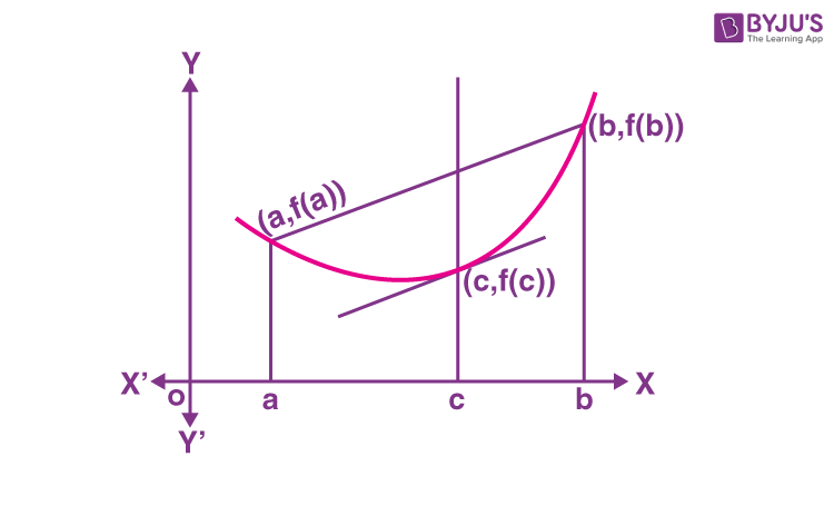
In the given graph the curve y = f(x) is continuous from x = a and x = b and differentiable within the closed interval [a,b] then according to Lagrange’s mean value theorem, for any function that is continuous on [a, b] and differentiable on (a, b) then there exists some c in the interval (a, b) such that the secant joining the endpoints of the interval [a, b] is parallel to the tangent at c.
This can be understood in a better way with the example given below.
Example:
Verify Mean Value Theorem for the function f(x) = x2 – 4x – 3 in the interval [a, b], where a = 1 and b = 4.
Solution:
Given,
f(x) = x2 – 4x – 3
f'(x) = 2x – 4
a = 1 and b = 4 (given)
f(a) = f(1) = (1)2 – 4(1) – 3 = 1 – 4 – 3 = -6
f(b) = f(4) = (4)2 – 4(4) – 3 = -3
Now,
[f(b) – f(a)]/ (b – a) = (-3 + 6)/(4 – 1) = 3/3 = 1
As per the mean value theorem statement, there is a point c ∈ (1, 4) such that f'(c) = [f(b) – f(a)]/ (b – a), i.e. f'(c) = 1.
2c – 4 = 1
2c = 5
c = 5/2 ∈ (1, 4)
Verification: f'(c) = 2(5/2) – 4 = 5 – 4 = 1
Hence, verified the mean value theorem.
Rolle’s Theorem
A special case of Lagrange’s mean value theorem is Rolle’s Theorem which states that:
If a function f is defined in the closed interval [a, b] in such a way that it satisfies the following conditions.
i) The function f is continuous on the closed interval [a, b]
ii)The function f is differentiable on the open interval (a, b)
iii) Now if f (a) = f (b) , then there exists at least one value of x, let us assume this value to be c, which lies between a and b i.e. (a < c < b ) in such a way that f‘(c) = 0 .
Precisely, if a function is continuous on the closed interval [a, b] and differentiable on the open interval (a, b) then there exists a point x = c in (a, b) such that f'(c) = 0
Geometric interpretation of Rolle’s Theorem
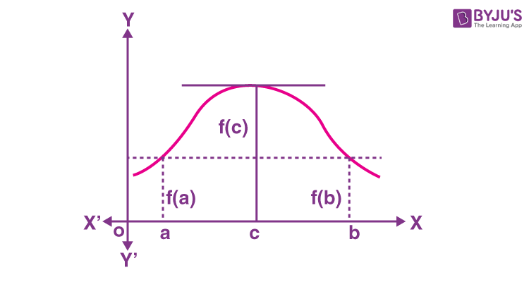
In the given graph, the curve y = f(x) is continuous between x =a and x = b and at every point, within the interval, it is possible to draw a tangent and ordinates corresponding to the abscissa and are equal then there exists at least one tangent to the curve which is parallel to the x-axis.
Algebraically, this theorem tells us that if f (x) is representing a polynomial function in x and the two roots of the equation f(x) = 0 are x =a and x = b, then there exists at least one root of the equation f‘(x) = 0 lying between these values.
The converse of Rolle’s theorem is not true and it is also possible that there exists more than one value of x, for which the theorem holds good but there is a definite chance of the existence of one such value.
Rolle’s Theorem Statement
Mathematically, Rolle’s theorem can be stated as:
Let f : [a, b] → R be continuous on [a, b] and differentiable on (a, b), such that f(a) = f(b), where a and b are some real numbers. Then there exists some c in (a, b) such that f′(c) = 0.
Rolle’s Theorem Example
Example:
Verify Rolle’s theorem for the function y = x2 + 2, a = –2 and b = 2.
Solution:
From the definition of Rolle’s theorem, the function y = x2 + 2 is continuous in [– 2, 2] and differentiable in (– 2, 2).
From the given,
f(x) = x2 + 2
f(-2) = (-2)2 + 2 = 4 + 2 = 6
f(2) = (2)2 + 2 = 4 + 2= 6
Thus, f(– 2) = f( 2) = 6
Hence, the value of f(x) at –2 and 2 coincide.
Now, f'(x) = 2x
Rolle’s theorem states that there is a point c ∈ (– 2, 2) such that f′(c) = 0.
At c = 0, f′(c) = 2(0) = 0, where c = 0 ∈ (– 2, 2)
Hence verified.
This is all about the mean value theorem and Rolle’s theorem. Explore more concepts of Differential Calculus with BYJU’S.

Comments