The standard normal distribution is one of the forms of the normal distribution. It occurs when a normal random variable has a mean equal to zero and a standard deviation equal to one. In other words, a normal distribution with a mean 0 and standard deviation of 1 is called the standard normal distribution. Also, the standard normal distribution is centred at zero, and the standard deviation gives the degree to which a given measurement deviates from the mean.
The random variable of a standard normal distribution is known as the standard score or a z-score. It is possible to transform every normal random variable X into a z score using the following formula:
z = (X – μ) / σ
where X is a normal random variable, μ is the mean of X, and σ is the standard deviation of X. You can also find the normal distribution formula here. In probability theory, the normal or Gaussian distribution is a very common continuous probability distribution.
Also, read:
Standard Normal Distribution Table
The standard normal distribution table gives the probability of a regularly distributed random variable Z, whose mean is equivalent to 0 and the difference equal to 1, is not exactly or equal to z. The normal distribution is a persistent probability distribution. It is also called Gaussian distribution. It is pertinent for positive estimations of z only.
A standard normal distribution table is utilized to determine the region under the bend (f(z)) to discover the probability of a specified range of distribution. The normal distribution density function f(z) is called the Bell Curve since its shape looks like a bell.
What does it mean? Is that on the off chance that you need to discover the probability of a value is not exactly or more than a fixed positive z value. You can discover it by finding it on the table. This is known as area Φ.
A standard normal distribution table presents a cumulative probability linked with a particular z-score. The rows of the table represent the whole number and tenth place of the z-score. The columns of the table represent the hundredth place. The cumulative probability (from –∞ to the z-score) arrives in the cell of the table.
For example, a part of the standard normal table is given below. To find the cumulative probability of a z-score equal to -1.21, cross-reference the row containing -1.2 of the table with the column holding 0.01. The table explains that the probability that a standard normal random variable will be less than -1.21 is 0.1131; that is, P(Z < -1.21) = 0.1131. This table is also called a z-score table.
| z | 0.00 | 0.01 | 0.02 | 0.03 | 0.04 | 0.05 |
| -3.0 | 0.0013 | 0.0013 | 0.0013 | 0.0012 | 0.0012 | 0.0011 |
| … | … | … | … | … | … | … |
| -1.4 | 0.0808 | 0.0793 | 0.0778 | 0.0764 | 0.0749 | 0.0735 |
| -1.3 | 0.0968 | 0.0951 | 0.0934 | 0.0918 | 0.0901 | 0.0885 |
| -1.2 | 0.1151 | 0.1131 | 0.1112 | 0.1093 | 0.1075 | 0.1056 |
| … | … | … | … | … | … | … |
| 3.0 | 0.9987 | 0.9987 | 0.9987 | 0.9988 | 0.9988 | 0.9989 |
Area of Standard Normal Distribution
Diagrammatically, the probability of Z not exactly “a” being Φ(a), figured from the standard normal distribution table, is demonstrated as follows: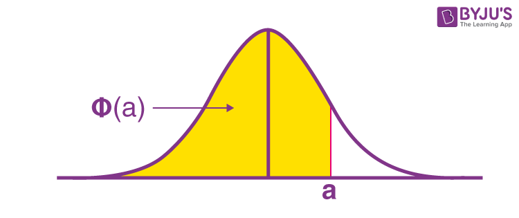
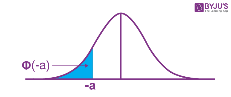
P(Z < –a)
As specified over, the standard normal distribution table just gives the probability to values, not exactly a positive z value (i.e., z values on the right-hand side of the mean). So how would we ascertain the probability beneath a negative z value (as outlined below)?
P(Z > a)
The probability of P(Z > a) is 1 – Φ(a). To understand the reasoning behind this look at the illustration below: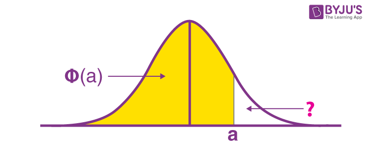
You know Φ(a), and you realize that the total area under the standard normal curve is 1 so by numerical conclusion: P(Z > a) is 1 Φ(a).
P(Z > –a)
The probability of P(Z > –a) is P(a), which is Φ(a). To comprehend this, we have to value the symmetry of the standard normal distribution curve. We are attempting to discover the region
Below:
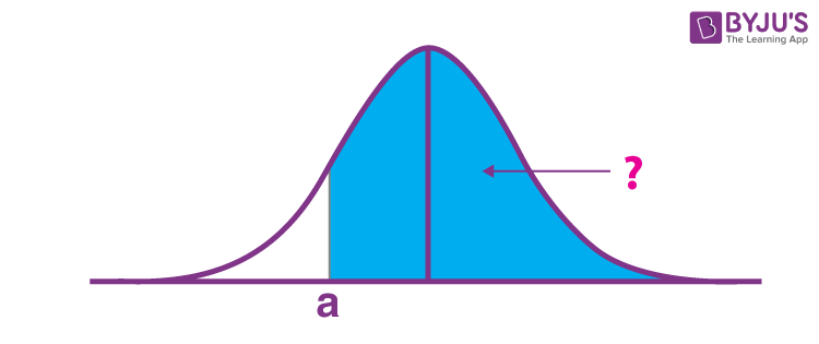
If this area is in the region we need.
Notice this is the same size area as the area we are searching for, just we know this area, as we can get it straight from the standard normal distribution table: it is
P(Z < a). In this way, the P(Z > –a) is P(Z < a), which is Φ(a).
Probability between z values
Let us find the probability between the values of z, i.e., a and b.
Consider the graph given below:
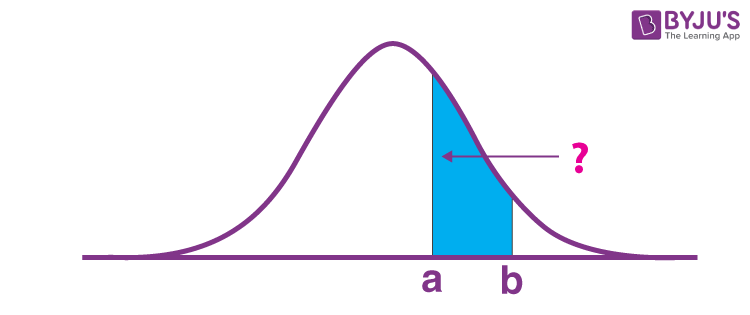
Now,
P(Z < b) – P(Z < a) = Φ(b) – Φ(a)
Thus,
P(a < Z < b) = Φ(b) – Φ(a)
Here, the values of a and b are positive.
Standard Normal Distribution Function
The standard normal distribution function for a random variable x is given by:
Probability Density Function is given by the formula,
This is a special case when μ = 0 and σ = 1. This situation of a normal distribution is also called the standard normal distribution or unit normal distribution.
Cumulative Distribution Function
The cumulative distribution function (CDF) of the standard normal distribution is generally denoted with the capital Greek letter Φ and is given by the formula:
Standard Normal Distribution Uses
- The standard normal distribution is a tool to translate a normal distribution into numbers. We may use it to get more information about the data set than was initially known.
- Standard normal distribution allows us to quickly estimate the probability of specific values befalling in our distribution or compare data sets with varying means and standard deviations.
- Also, the z-score of the standard normal distribution is interpreted as the number of standard deviations a data point falls above or below the mean.
Characteristics of Standard Normal Distribution
A z-score of a standard normal distribution is a standard score that indicates how many standard deviations are away from the mean an individual value (x) lies:
- When z-score is positive, the x-value is greater than the mean
- When z-score is negative, the x-value is less than the mean
- When z-score is equal to 0, the x-value is equal to the mean
The empirical rule, or the 68-95-99.7 rule of standard normal distribution, tells us where most values lie in the given normal distribution. Thus, for the standard normal distribution, 68% of the observations lie within 1 standard deviation of the mean; 95% lie within two standard deviations of the mean; 99.7% lie within 3 standard deviations of the mean.
Normal Distribution-Real World Example
Usually, happenings in the real world follow a normal distribution. This enables researchers to practice normal distribution as a model for evaluating probabilities linked with real-world scenarios. Basically, the analysis includes two steps:
- Converting raw data into the form of z-score, using the conversion equation given as z = (X – μ) / σ.
- Finding the probability. After the raw data is transformed into z-scores, then with the help of standard normal distribution tables or normal distribution calculators available online to find probabilities linked with the z-scores.
Standard Normal Distribution Problem and Solution
Problem 1: For some computers, the time period between charges of the battery is normally distributed with a mean of 50 hours and a standard deviation of 15 hours. Rohan has one of these computers and needs to know the probability that the time period will be between 50 and 70 hours.
Solution: Let x be the random variable that represents the time period.
Given Mean, μ= 50
and standard deviation, σ = 15
To find: Pprobability that x is between 50 and 70 or P( 50< x < 70)
By using the transformation equation, we know;
z = (X – μ) / σ
For x = 50 , z = (50 – 50) / 15 = 0
For x = 70 , z = (70 – 50) / 15 = 1.33
P( 50< x < 70) = P( 0< z < 1.33) = [area to the left of z = 1.33] – [area to the left of z = 0]
From the table we get the value, such as;
P( 0< z < 1.33) = 0.9082 – 0.5 = 0.4082
The probability that Rohan’s computer has a time period between 50 and 70 hours is equal to 0.4082.
Problem 2: The speeds of cars are measured using a radar unit, on a motorway. The speeds are normally distributed with a mean of 90 km/hr and a standard deviation of 10 km/hr. What is the probability that a car selected at chance is moving at more than 100 km/hr?
Solution: Let the speed of cars is represented by a random variable ‘x’.
Now, given mean, μ = 90 and standard deviation, σ = 10.
To find: Probability that x is higher than 100 or P(x > 100)
By using the transformation equation, we know;
z = (X – μ) / σ
Hence,
For x = 100 , z = (100 – 90) / 10 = 1
P(x > 90) = P(z > 1) = [total area] – [area to the left of z = 1]
P(z > 1) = 1 – 0.8413 = 0.1587


Comments