Axiomatic Probability

In the normal approach to probability, we consider random experiments, sample space and other events that are associated with the different experiments. In our day to day life, we are more familiar with the word ‘chance’ as compared to the word ‘probability’. Since Mathematics is all about quantifying things, the theory of probability basically quantifies these chances of occurrence or non-occurrence of the events. There are different types of events in probability. Here, we will have a look at the definition and the conditions of the axiomatic probability in detail.

Axiomatic Probability Definition

One important thing about probability is that it can only be applied to experiments where we know the total number of outcomes of the experiment, i.e. unless and until we know the total number of outcomes of an experiment, concept of probability cannot be applied.

Thus, in order to apply probability in day to day situations, we should know the total number of possible outcomes of the experiment. Axiomatic Probability is just another way of describing the probability of an event. As, the word itself says, in this approach, some axioms are predefined before assigning probabilities. This is done to quantize the event and hence to ease the calculation of occurrence or non-occurrence of the event.

Axiomatix Probability Conditions

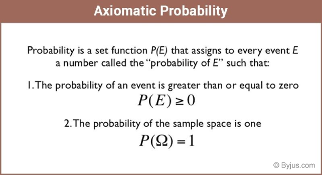
Let, S be the sample space of any random experiment and let

1. For any event
   \(\begin{array}{l}E\end{array} \)
   ,
   \(\begin{array}{l}P(E) ≥ 0\end{array} \)
2. \(\begin{array}{l}P(S)\end{array} \)
   =
   \(\begin{array}{l}1\end{array} \)
3. In case
   \(\begin{array}{l}E\end{array} \)
   and
   \(\begin{array}{l}F\end{array} \)
   are mutually exclusive events, then following equation will be valid:
   \(\begin{array}{l}P(E ∪ F)\end{array} \)
   =
   \(\begin{array}{l}P(E) + P(F)\end{array} \)

From point (3) it can be stated that

If we need to prove this, let us take

P(E ∪ ф) = P(E) + P(ф) or

P(E)=P(E) + P(ф)

i.e.P(ф)=0

Let, the sample space of S contain the given outcomes

1. \(\begin{array}{l}0 ≤ P(δ_i) ≤ 1\end{array} \)
   for each
   \(\begin{array}{l}δ_i ∈ S\end{array} \)
2. \(\begin{array}{l}P(δ_1) + P(δ_2)+ … + P(δ_n)\end{array} \)
   =
   \(\begin{array}{l}1\end{array} \)
3. For any event
   \(\begin{array}{l}Q\end{array} \)
   ,
   \(\begin{array}{l}P(Q)\end{array} \)
   =
   \(\begin{array}{l}∑P(δ_i), δ_i ∈ Q\end{array} \)
   .

This is to be noted that the singleton {

Axiomatic Probability Example

Now let us take a simple example to understand the axiomatic approach to probability.

On tossing a coin we say that the probability of occurrence of head and tail is

This condition basically satisfies both the conditions, i.e.

• Each value is neither less than zero nor greater than 1 and
• Sum of the probabilities of occurrence of head and tail is 1

Hence, for this case we can say that the probabilities of occurrence of head and tail are

Now, say

Does this probability value satisfy the conditions of axiomatic approach?

For this, let us again check the basic initial conditions of the axiomatic approach of probability.

• Each value is neither less than zero nor greater than 1 and
• Sum of the probabilities of occurrence of head and tail is 1

Hence this sort of probability value assignment also satisfies the axiomatic approach of probability. Thus, we can conclude that there can be infinite ways to assign the probability to outcomes of an experiment.

Please log on to www.byjus.com to know more. Relish the joy of learning with us.