In mathematics, an autonomous system is a system of ODEs (ordinary differential equations) that do not explicitly depend on the independent variable. It is also called an autonomous differential equation. When the time is taken as a variable, they are also called invariant time systems. Planar autonomous systems of ordinary differential equations play an important role in mathematics and physics. In this article, you will learn in detail about the planar autonomous system of ODE, along with some basic concepts related to this.

Learn: Ordinary differential equations

Planar Autonomous System

A set of two scalar ordinary differential equations of the form x'(t) = F(x(t), y(t)) and y'(t) = G(x(t), y(t)) is called a planar autonomous system of ODEs. Here, the term autonomous means representative which is justified by the lack of t, i.e., the time variable in the functions F(x, y) and G(x, y).

We can estimate various elements through the solution of a planar autonomous system of linear PDEs, such as traces, trajectories, phase portrait, and so on.

Trace:

Let (x(t), y(t)) be the solution of a planar (i.e., two-dimensional) autonomous system of PDEs. So, the trace of (x(t), y(t)) as t varies will be a curve in the plane. This curve is also called an orbit or trajectory.

Trajectory:

A trajectory is a graph of the solution to an ordinary differential equation. Trajectories may also be called paths.

Phase Portrait:

A Phase Portrait of a system of ordinary differential equations is a collection of trajectories of the system.

How to Solve Planar Autonomous System of Linear ODEs?

Now, let’s understand how to solve a planar autonomous system of linear ordinary differential equations to get various results such as eigenvalues, eigenvectors, and so on, with the help of a solved example given below.

Example:

Consider the planar linear autonomous system of ordinary differential equations:

dx/dt = ax + by

dy/dt = bx + ay; a < 0 and b > 0

Now, calculate the following parameters.

(i) Using the trace and determinant of the coefficient matrix, find the eigenvalues and the corresponding eigenvectors of the associated matrix.

(ii) If a² < b², then determine how the given system is classified in the trace determinant plane?

(iii) If a² > b², then determine how the given system is classified in the trace determinant plane?

(iv) Draw a phase portrait for one of the cases a² < b² or a² > b².

(i) Finding the Eigenvalues and Eigenvectors

Let the eigenvalues be α and β.

We know that the trace of a matrix can be defined in two ways: the sum of the diagonal elements and second by the sum of the eigenvalues. Using these two equivalent definitions, we get:

α + β = 2a…..(1)

Next, we know that the determinant of a matrix is also the product of its eigenvalues, so, this gives: αβ = a² – b²…..(2)

Solving for α and β:

As we know, (α – β)² = (α + β)² – 4αβ

= (2a)² – 4(a² – b²)

= 4a² – 4a² + 4b²

= 4b²

So, α – β = ±2b…..(3)

From equations (1) and (3), we get the eigenvalues as (a + b) and (a – b).

Eigenvector for the eigenvalue (a + b):

In this case, we can write the given system of equations as:

From this, we get the corresponding elements as:

ax + by = ax + bx

And

bx + ay = ay + by

Simplification of the above equations will gives us x = y as b ≠ 0. {given b > 0}

Therefore, the eigenvector for the eigenvalue (a + b) =

Eigenvector for the eigenvalue (a – b):

In this case, we can write the given system of equations as:

From this, we get the corresponding elements as:

ax + by = ax – bx

And

bx + ay = ay – by

Simplification of the above equations will gives us y = -x as b ≠ 0. {given b > 0}

Therefore, the eigenvector for the eigenvalue (a – b) =

(ii) System in the trace determinant plane when a² < b²

We know that the determinant of the coefficient matrix of the linear system is a² – b².

That means,

If a² < b², then |A| < 0.

So, a² – b² < 0

Let D be the determinant and T be the trace.

So, the quantity T² – 4D = b² > 0.

Hence, the eigenvalues are real and distinct (from the calculation above).

Also, a² – b² < 0

⇒ (a + b)(a – b) < 0

Thus, the eigenvalues possess opposite signs.

That means along the direction of one eigenvector, the flow converges towards the origin, and along the direction of another eigenvector, the flow diverges away from the origin. So, this is the case of the saddle. The region represented in the trace-determinant plane will be the entire half-plane below the trace axis.

(iii) System in the trace determinant plane when a² > b²

As a² > b², so we have a² – b² > 0

⇒ (a + b)(a – b) > 0

So, both the eigenvalues have the same sign.

From the given, we have a < 0 and b > 0.

So, we must contain a – b < 0.

That means both the eigenvalues are negative. Thus, we have a nodal sink.

The above two cases can be shown graphically as:

(iv) Phase portrait for one of the cases a² < b² or a² > b².

To draw the phase portraits, when a² < b², we see that a + b > 0 and a – b < 0, i.e. the origin is a saddle point. Since the origin is a saddle, considering the eigenvalues, we see that there will be a linear flow along the direction of the eigenvector

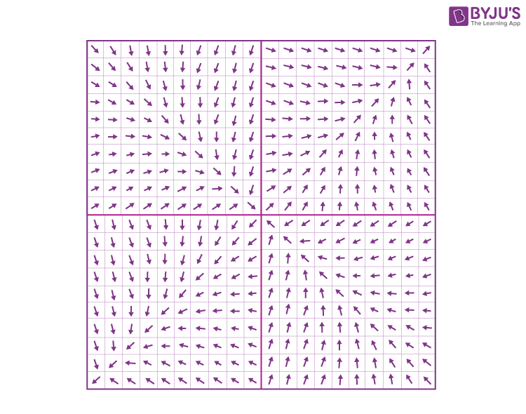
In the other case, a² > b², since both the eigenvalues are negative, and a – b < a + b < 0, the flow will move parallelly to the sink along the eigen direction of the smaller eigenvalue (a – b). And it will show turning along the eigen direction of the bigger eigenvalue (a + b). So, the flow will be as shown below:

To learn more about ordinary differential equations and their solutions, download BYJU’S – The Learning App today!