Magnetic Field - Definition, Formula, Measurement, Units, Magnetic Force

A magnetic field is an invisible space around a magnetic object. It is basically used to describe the distribution of magnetic force around a magnetic object.

Magnetic fields are created or produced when the electric charge/current moves within the vicinity of the magnet. Here, the sub-atomic particle, such as electrons with a negative charge, moves around, creating a magnetic field. These fields can originate inside the atoms of magnetic objects or within electrical conductors or wires.

Representation of Magnetic Field
Magnetic Field Unit
Magnetic Force
Magnetic Field of a Straight Line Current
Magnetic Field of a Current-carrying Circular Loop
Magnetic Field Variation on the Axial Distance
Magnetic Field of a Solenoid

Representation of Magnetic Field

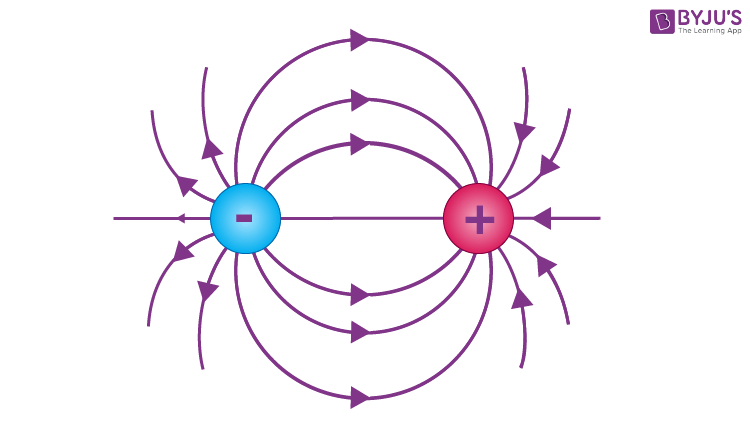
A magnetic field can be depicted in several ways. Mathematically, it can be represented as a vector field which can be plotted as different sets on a grid. Another way is the use of field lines. The set of vectors is connected with lines. Here, the magnetic field lines never cross each other and never stop.

Magnetic Field

Magnetic Field Unit and Measurement

The measurement of the magnetic field involves measuring its strength and direction. The measurement is necessary because every magnetic field is different from each other. While some magnetic field intensity is small and weak, others are very strong and large. If we look at the earth’s magnetic field, it is weak but large.

Also Read: Electromagnetism

Nonetheless, the term magnetic field represents two unique but related fields which are usually denoted by the symbols H and B. H represents the magnetic field strength and is measured in the SI unit of an ampere per metre. Meanwhile, B represents magnetic flux density and is measured in tesla.

Magnetic Force

A magnetic field depicts how a moving charge flows around a magnetic object. Magnetic force is a force that arises due to the interaction of magnetic fields. It can be either a repulsive or attractive force.

Magnetic Force Acting on a Moving Charge in the Presence of a Magnetic Field

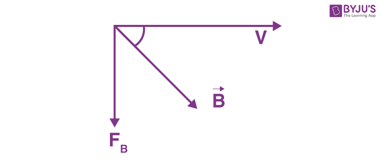
A change ‘a’ is moving with a velocity ‘v’, making an angle ‘θ’ with the field direction. Experimentally, we found that a magnetic force acts on the moving charge and is given by

\(\begin{array}{l}{{\overrightarrow{F}}_{B}}=q\left( \overrightarrow{V}\times \overrightarrow{B} \right).\end{array} \)

This is known as the Lorentz force law.

Lorentz Force Law

Characteristics

(1) No magnetic force acts on a stationary change present in the magnetic field.

(2) No magnetic force acts on a moving change when it is moving either parallel (or) antiparallel to the field direction.

(3) The magnetic force acting on the moving change is maximum,

\(\begin{array}{l}\text{when the change is moving}\bot ar\ \text{to}\ \overrightarrow{B}.\end{array} \)

So, as

\(\begin{array}{l}\overrightarrow{V}\bot \overrightarrow{B},\,\theta =90{}^\circ \Rightarrow \overrightarrow{{{F}_{B}}}=\text{maximum}.\end{array} \)

No work is done by the magnetic force on a moving charge because

\(\begin{array}{l}\overrightarrow{{{F}_{B}}}\ \text{is always}\ \bot ar\,to\,\overrightarrow{B}.\end{array} \)

As a result, there is no change in K.E. of a change. There is no change in speed, but the direction of motion may change.

Magnetic Force on Currents

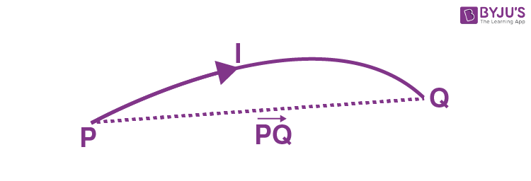
Let us consider a line charge ‘λ’ moving with a velocity ‘v’, as shown in the figure. The amount of charge crossing a point p in a time interval Δt is λVΔt. The rate of flow of charge across point p is nothing but the line current I.

\(\begin{array}{l}I=\frac{\lambda V \Delta t}{\Delta t}=\lambda V\,\,\,;\,\,\overrightarrow{I}=\overrightarrow{\lambda V}(In\,vector\,form)\end{array} \)

⇒ A change moving with a velocity ‘v’ (a discrete change, line change, surface change (or) volume change) is equivalent to the current. The force acting on a line change moving with a velocity ‘v’ (or) the magnetic force acting on a line current is given by

\(\begin{array}{l}\overrightarrow{F}=\int\limits_{L}{\left( \overrightarrow{V}\times \overrightarrow{B} \right)dq=\int\limits_{L}{\left( \overrightarrow{V}\times \overrightarrow{B} \right)\lambda d\ell .}}=\,\int\limits_{L}{\left( \overrightarrow{I}\times \overrightarrow{B} \right)d\ell }=I\int\limits_{L}{\left( \overrightarrow{d\ell }\times \overrightarrow{B} \right)}\end{array} \)

Note: I is taken out of the integral because the currents which we are considering are study currents.

\(\begin{array}{l}\text{A conductor}\ \overrightarrow{PQ}\ \text{is carrying a current}\ ^{‘}I'\end{array} \)

& is present in a magnetic field.

Magnetic Force on Currents

\(\begin{array}{l}\overrightarrow{F}=I\int\limits_{P}^{Q}{d\overrightarrow{\ell }\times \overrightarrow{B}}\end{array} \)

\(\begin{array}{l}\text{If}\ \overrightarrow{B}\ \text{is uniform,}\end{array} \)

\(\begin{array}{l}\overrightarrow{F}=I\left[ \int\limits_{P}^{Q}{\overrightarrow{d\ell }} \right]\left. \times \overrightarrow{B} \right]=I\left[ \overrightarrow{PQ}\times \overrightarrow{B} \right]\end{array} \)

If it is a closed current-carrying conductor, carrying a steady current

\(\begin{array}{l}\text{and is placed in a magnetic field}\ \overrightarrow{B}.\end{array} \)

\(\begin{array}{l}\overrightarrow{F}=I\oint\limits_{L}{\overrightarrow{d\ell }}\times \overrightarrow{B}\end{array} \)

\(\begin{array}{l}\text{If}\ \overrightarrow{B}\ \text{is uniform, then}\end{array} \)

the magnetic force acting on it is always equal to zero.

Magnetic Field of a Straight Line Current

A straight current-carrying conductor is carrying a current I, as shown in the figure. By using Biot-Savart’s law, we are now finding the magnetic field at a point p, which is at a distance ‘r’ from the wire.

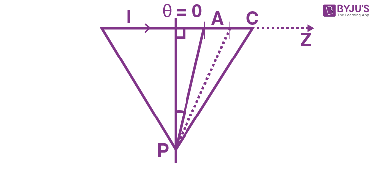
Magnetic Field Of A Straight Line Current

\(\begin{array}{l}OA = Z\cos \theta =\frac{r}{PA}\end{array} \)

r tanθ = Z

dz = r sec²θ dθ

\(\begin{array}{l}PA=r\sec \theta\end{array} \)

\(\begin{array}{l}dB=\frac{{{\mu }_{o}}Idz\,\sin \angle PAC}{4\pi {{(PA)}^{2}}}\end{array} \)

Magnetic Field Of A Straight Line Current

\(\begin{array}{l}=\frac{{{\mu }_{o}}I\, r\sec^{2}\theta\, d\theta\, \cos \theta }{4\pi \left( r^{2}\sec^{2}\theta \right)}=\frac{{{\mu }_{o}}I\cos \theta d\theta }{4\pi r}\end{array} \)

\(\begin{array}{l}=\overrightarrow{B}=\frac{{{\mu }_{o}}I}{4\pi r}\int\limits_{-{{\theta }_{1}}}^{{{\theta }_{2}}}{\cos \theta d\theta }\end{array} \)

\(\begin{array}{l}=\frac{{{\mu }_{o}}I}{4\pi r}\left( \sin ({{\theta }_{1}})+sin({{\theta }_{2}}) \right)\end{array} \)

Case I: In the case of an infinite wire carrying a current I, the angle subtended by the ends at the point P can be considered

\(\begin{array}{l}{{\theta }_{1}}={{\theta }_{2}}=\frac{\pi }{2}\end{array} \)

\(\begin{array}{l}\Rightarrow \,\overrightarrow{B}=\frac{{{\mu }_{o}}I}{4\pi r}(2)=\frac{{{\mu }_{o}}I}{2\pi r}\end{array} \)

Case II: If the wire has a length extended to ∞, and the point P is present on a perpendicular passing through one end of this semi-infinite wire.

Magnetic Field Of A Straight Line Current

\(\begin{array}{l}=\frac{{{\mu }_{o}}I}{4\pi r}\left( \sin ({{\theta }_{1}})+sin({{\theta }_{2}}) \right)\end{array} \)

\(\begin{array}{l}{{\theta }_{1}}=0{}^\circ ,{{\theta }_{2}}=90{}^\circ\end{array} \)

\(\begin{array}{l}\Rightarrow \,\overrightarrow{B}=\frac{{{\mu }_{o}}I}{4\pi r}\end{array} \)

Case III: If the point p is on a ⊥ar bisector of length 2L.

\(\begin{array}{l}\overrightarrow{B}=\frac{{{\mu }_{o}}I}{4\pi r}\left( 2Sin\theta \right)=\frac{{{\mu }_{o}}ISin\theta }{2\pi r}\end{array} \)

(or)

\(\begin{array}{l}\overrightarrow{B}=\frac{{{\mu }_{o}}I}{2\pi r}\frac{L}{\sqrt{{{L}^{2}}+{{r}_{2}}}}\end{array} \)

Magnetic Field Of A Straight Line Current

Magnetic Field of a Current-carrying Circular Loop

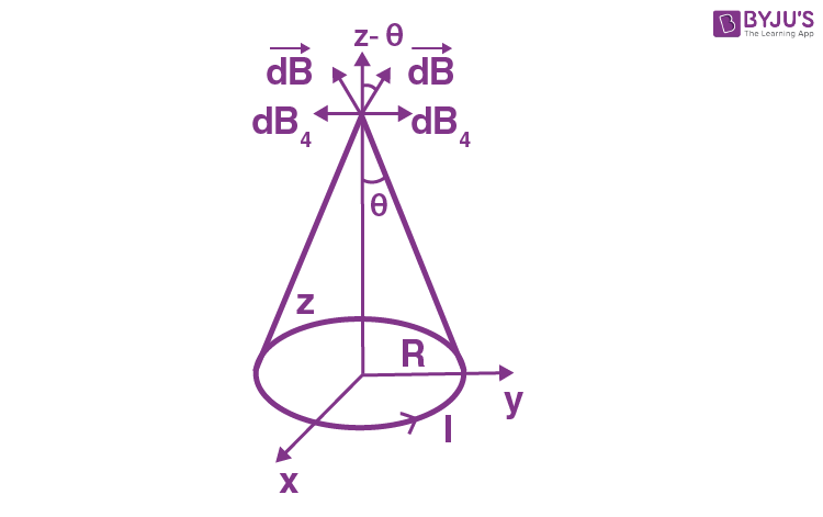
A circular loop carrying a current I in an anti-clockwise direction lies in XY-plane with its centre at the origin. By using B.S.L., we are now calculating a magnetic field at point P.

Using B.S.L.,

\(\begin{array}{l}\overrightarrow{dB}=\frac{{{\mu }_{o}}}{4\pi }\frac{Id\ell \sin \theta }{({{R}^{2}}+{{z}^{2}})}\end{array} \)

In case of a circular loop,

\(\begin{array}{l}\overrightarrow{d\ell }\ \text{and}\ \hat{r}\ \text{are perpendicular}.\end{array} \)

\(\begin{array}{l}\therefore \overrightarrow{dB}=\frac{{{\mu }_{o}}}{4\pi }\frac{id\ell }{({{R}^{2}}+{{z}^{2}})}\end{array} \)

\(\begin{array}{l}\text{The y – components of}\ \overrightarrow{dB}\ \text{are cancelling each other. }\end{array} \)

\(\begin{array}{l}\text{The}\ \overrightarrow{B}\ \text{is contributed only by z-components}\ {{\overrightarrow{dB}}_{z}}.\end{array} \)

\(\begin{array}{l}\overrightarrow{B}=\oint{d{{B}_{z}}=\hat{z}}\int{\overrightarrow{dB}\,sin\theta }=\hat{z}\oint{\frac{{{\mu }_{o}}}{4\pi }\frac{Id\ell }{{{R}^{2}}+{{z}^{2}}}}\,\frac{R}{{{({{R}^{2}}+{{z}^{2}})}^{\frac{1}{2}}}}\end{array} \)

\(\begin{array}{l}=\hat{z}\frac{{{\mu }_{o}}}{4\pi }\,\frac{IR}{{{\left( {{R}^{2}}+{{z}^{2}} \right)}^{{}^{3}/{}_{2}}}}\oint{d\ell }\end{array} \)

\(\begin{array}{l}=\hat{z}\frac{{{\mu }_{o}}IR(2\pi R)}{4\pi {{({{R}^{2}}+{{z}^{2}})}^{{}^{3}/{}_{2}}}}=\hat{z}\frac{{{\mu }_{o}}I}{2R{{\left[ 1+\frac{{{z}^{2}}}{{{R}^{2}}} \right]}^{{}^{3}/{}_{2}}}}\end{array} \)

At the centre, z = 0,

\(\begin{array}{l}\overline{B}=\frac{{{\mu }_{o}}I}{2R}\hat{z}\end{array} \)

A circular loop, carrying a current I, behaves as a magnetic dipole having magnetic dipole moment

\(\begin{array}{l}(m)\overrightarrow{m}=I\int\limits{da}.\end{array} \)

In the case of flat surfaces, m = I (πR²)

\(\begin{array}{l}\overrightarrow{B}=\hat{z}\frac{{{\mu }_{o}}m}{2\pi {{({{R}^{2}}+{{z}^{2}})}^{{}^{3}/{}_{2}}}}\left( \overrightarrow{B}\ \text{of dipole one axial line} \right)\end{array} \)

The direction of the magnetic dipole moment depends on the sense that the current in the loop is in the anti-clockwise direction, then ‘m’ is directed ⊥ar to the plane outwards. If the current is in a clockwise direction, then the magnetic moment is directed ⊥ar to the plane inwards.

Magnetic Field Variation on the Axial Distance

At the centre, the M.F. is maximum, but when we are moving to either side of the circular loop along the z-axis, the field varies non-linearly at two points along the axis,

\(\begin{array}{l}\text{the second derivative of}\ \overrightarrow{B}\ \text{is vanishing and becoming zero.}\end{array} \)

Magnetic Field Variation on the Axial Distance

\(\begin{array}{l}\text{The variation of}\ \overrightarrow{B}\ \text{with Z is constant at these two-points}.\end{array} \)

\(\begin{array}{l}\text{The variation of}\ \overrightarrow{B}\ \text{is linear at the two points.}\end{array} \)

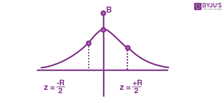
These two points are known as ‘the points of inflexion of the graph’.

Magnetic Field of a Solenoid

Magnetic Field Of A Solenoid

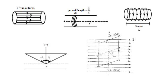
‘N’ turns are wound on a cylindrical tube having radius ‘a’ and length ‘L’ so closely that the surface of the cylindrical tube presents a surface current density ‘k’, assuming each turn has a circular shape.

The M.F. on the axis due to each turn carrying a current I is

\(\begin{array}{l}\overrightarrow{B}=\frac{{{\mu }_{o}}I{{R}^{2}}}{2{{({{R}^{2}}+{{z}^{2}})}^{3/2}}}\end{array} \)

In a length dz.

The number of turns is n d z, and the current I in the above formula can be replaced by ndzi of the M.F. due to this current.

\(\begin{array}{l}\overrightarrow{dB}=\frac{{{\mu }_{o}}ndzi{{a}^{2}}}{2{{({{a}^{2}}+{{z}^{2}})}^{{}^{3}/{}_{2}}}}\end{array} \)

z = a tan θ , dx = a sec²θ dθ.

\(\begin{array}{l}dB=\frac{{{\mu }_{o}}ni{{a}^{2}}}{2}\left[ \frac{a{{\sec }^{2}}\theta d\theta }{{{a}^{3}}{{\left[ 1+{{\tan }^{2}}\theta \right]}^{{}^{3}/{}_{2}}}} \right]=\frac{{{\mu }_{o}}ni{{a}^{3}}{{\sec }^{2}}\theta d\theta }{2{{a}^{3}}{{\sec }^{3}}\theta }=\frac{{{\mu }_{o}}ni}{2\sec \theta }d\theta\end{array} \)

\(\begin{array}{l}dB=\frac{{{\mu }_{o}}ni}{2}\cos \theta d\theta\end{array} \)

This is the M.F. due to the small surface current element dz of the surface current at a point p on the axis.

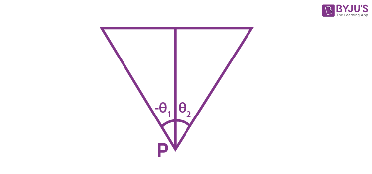
If the two ends of the solenoid are subtending angles, θ₁ and θ₂, at the point p on the axis of the solenoid, then the M.F. at point p is given by

\(\begin{array}{l}\overrightarrow{B}=\frac{{{\mu }_{o}}ni\hat{z}}{2}\int\limits_{-{{\theta }_{1}}}^{{{\theta }_{2}}}{\cos \theta d\theta }\end{array} \)

\(\begin{array}{l}=\frac{{{\mu }_{o}}ni}{2}\left[ sin{{\theta }_{1}}+sin{{\theta }_{2}} \right]\end{array} \)

\(\begin{array}{l}= \frac{\mu_o ni }{2}[sin\theta_1 + sin\theta_2 ]\hat{\not{Z}}\end{array} \)

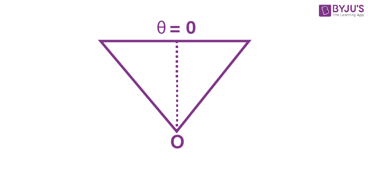
Case I: For a long solenoid at any point O inside the solenoid, the M.F. can be calculated as follows:

\(\begin{array}{l}\overrightarrow{B}=\,\frac{{{\mu }_{o}}ni}{2}(2)={{\mu }_{o}}ni\overset{ˆ}{\mathop{z}}\,\,\,\,\,\,\,\,\,\,\,\,\,\,\,\,\,\,\,\to 1\end{array} \)

Case II: If the point P is at one end of the long solenoid.

\(\begin{array}{l}{{\theta }_{1}}=0,{{\theta }_{2}}=\frac{\pi }{2} \\\overrightarrow{B}=\overset{ˆ}{\mathop{z}}\,\frac{{{\mu}_{o}}ni}{2}\,\,\,\,\,\,\,\,\,\,\,\,\,\,\,\,\,\,\,\,\,\,\,\,\,\,\,\,\to 2 \\\end{array} \)

Comparing 1 and 2, the magnetic field is only 1/2 at the end because there is a leakage of ϕ_B at the ends. We can avoid this leakage of flux by joining the ends of the solenoid. This is called an endless solenoid (or) solenoid toroid.

Force and Torque on a Current Loop or Coil in a Uniform Magnetic Field

Let a rectangular current loop ABCD having length AB = CD = l and breadth AD = BC = b and carrying current ‘i’ be suspended in a magnetic field of flux density B. With normal (ON) to its plane, making an angle Ɵ with the field direction.

Forces I (b × B) on arms AD and BC act in opposite directions along the vertical axis of suspension X Y and hence, cancel.

Forces on arms AB and DC, being perpendicular to the field, are ilB each, and they act at the middle points P and Q, as shown in the figure.

Force and Torque on a Current Loop or Coil in a Uniform Magnetic Field

These forces form a couple of arms PR = PQ sin Ɵ = b sin Ɵ.

Torque = Force X arm or perpendicular distance between the two forces

\(\begin{array}{l}\tau = i\ell B\times b \sin \theta\end{array} \)

\(\begin{array}{l}= i(\ell B) B \sin \theta\end{array} \)

\(\begin{array}{l}= i(A) B \sin \theta\end{array} \)

\(\begin{array}{l}\;\;\;(Since\;\ell b = A)\end{array} \)

For a loop having n turns,

\(\begin{array}{l}or\,\tau =n\,i\,AB\sin \,\theta \,\,\,\,\,\,\,\,\,…..\,\end{array} \)

If the plane of the loop makes an angle Ɵ with the direction of B, then,

\(\begin{array}{l}\tau =n\,i\,AB\cos \,\theta\end{array} \)

It can be seen from the above equation that the torque acting on the coil is similar to the torque acting on a magnet in a uniform magnetic field,

\(\begin{array}{l}\,\tau =MB\sin \,\theta\end{array} \)

since the current loop behaves like a magnetic dipole of magnetic moment, M = niA.

When the plane of the circular loop is parallel to the applied magnetic field, the torque becomes maximum, i.e.,

\(\begin{array}{l}\,\tau =n\,i\,AB.\end{array} \)

When the plane of the circular loop is perpendicular to the applied magnetic field, the torque becomes minimum, i.e., τ = 0.

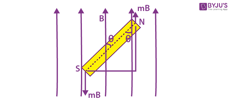
Couple Acting on a Bar Magnet Placed in a Uniform Magnetic Field

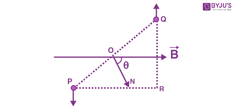
Let us consider a bar magnet (NS) of pole strength ‘m’ and magnetic length ‘2l‘, placed in a uniform magnetic field ‘B’, as shown in the figure, at an angle Ɵ to the direction of the field. Each pole of the magnet is then acted upon by a force equal to mB but in opposite directions. Thus, two equal and opposite forces act on the rigid body of the magnet at the ends, constituting a couple. This couple tends to rotate the magnet so as to bring it along the direction of the field.

The torque τ due to the couple or the moment of the couple is equal to the product of the force and the perpendicular distance between the two forces, and is given by

Couple Acting on a Bar Magnet Placed in a Uniform Magnetic Field

τ = (mB) SP = mB(NS) sin θ ( since sin θ = SP/NS)

(or) τ = mB (2l) sin θ (since NS = 2l)

= (m 2l) B sin θ

= MB sin θ

Where M = (m 2l) B sin θ is a constant for a given magnet and is known as the moment of the magnet; thus, the torque on the magnet depends on the angle between the magnetic field ‘B’ and the axis of the magnet. When the magnet is parallel to the direction of the field (θ = 0), the torque on the magnet is equal to zero. If the magnet is at right angles to the direction of the field (θ = 90°), the torque is maximum τ = mB.

Magnetic Induction Due to a Bar Magnet on Its Axial Line

The axial line of a magnet is the line passing through both poles of the magnet. Let us consider a bar magnet (NS) of magnetic length ‘2l’ and pole strength ‘m’, as shown in the figure.

Magnetic Induction Due to a Bar Magnet on its Axial Line

Let ‘A’ be a point on the axial line at a distance d from the centre (O) of the magnet. The magnetic induction at ‘A’ due to the north pole of the magnet is given by

\(\begin{array}{l}B_N = \frac{\mu_o}{4\pi}\frac{m}{(NA)^2} \end{array} \)

\(\begin{array}{l}B_N = \frac{\mu_o}{4\pi}\frac{m}{(d-\ell)^{2}} \end{array} \)

acting along NA.

Similarly, the magnetic induction at A due to the south pole of the magnet is given by

\(\begin{array}{l}B_s = \frac{\mu_o}{4\pi}\frac{m}{(SA)^2}\end{array} \)

\(\begin{array}{l}B_s = \frac{\mu_o}{4\pi}\frac{m}{(d+\ell)^2}\ \text{acting along AS}\end{array} \)

Therefore, the resultant magnetic induction at A is along NA, and is given by

\(\begin{array}{l}{{B}_{A}}={{B}_{N}}-{{B}_{S}}=\frac{{{\mu }_{0}}}{4\pi }\frac{m}{{{(d-\ell )}^{2}}}-\frac{{{\mu }_{0}}}{4\pi }\frac{m}{{{(d+\ell )}^{2}}}\,\,\,\,\,\,\, \\ \,\,\,\,\,\,\,\,\,\,\,\,or\,{{B}_{A}}=\left( \frac{{{\mu }_{0}}m}{4\pi } \right)\left[ \frac{1}{{{(d-\ell )}^{2}}}-\frac{1}{{{(d+\ell )}^{2}}} \right]=\frac{\mu 0}{4\pi }\frac{m.4d\ell }{{{({{d}^{2}}-{{\ell }^{2}})}^{2}}} \\\end{array} \)

\(\begin{array}{l}or\,{{B}_{A}}=\frac{{{\mu }_{0}}}{4\pi }\frac{m(2\ell )2d}{{{\left( {{d}^{2}}-{{\ell }^{2}} \right)}^{2}}}=\frac{{{\mu }_{0}}}{4\pi }\frac{2MD}{{{({{d}^{2}}-{{\ell }^{2}})}^{2}}}\,\,\,\,\,\,\,\,\,\,(Since, \; M=m2\ell )\end{array} \)

Where M = m (2l) is the magnetic moment of the magnet.

Thus, the magnetic induction at any point on the axial line of a bar magnet is given by

\(\begin{array}{l}\,{{B}_{A}}=\frac{{{\mu }_{0}}}{4\pi }\frac{2Md}{{{({{d}^{2}}-{{\ell}^{2}})}^{2}}}\end{array} \)

The direction of the magnetic induction B_A on the axial line is always in the same direction as the magnetic moment.

In the case of a short bar magnet, i.e., when l < < d, we can approximate the above equation as

\(\begin{array}{l}{{B}_{A}}=\frac{{{\mu }_{0}}}{4\pi }\frac{2M}{{{d}^{3}}}\end{array} \)

Magnetic Induction Due to a Bar Magnet on Its Equatorial Line

Magnetic Induction Due to a Bar Magnet on its Equatorial Line

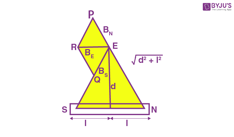
The equatorial line of a magnet is the perpendicular bisector of the axis of the magnet. Let us consider point E on the equatorial line of a bar magnet (NS) at a distance d from the centre ‘O’ of the magnet. Let ‘m’ be the pole strength and ‘2l’ be the distance between the two poles of the magnet.

The magnetic induction at ‘E’ due to the north pole of the magnet is given by

\(\begin{array}{l}{{B}_{N}}=\frac{{{\mu }_{0}}}{4\pi }\frac{m}{{{(NE)}^{2}}}=\frac{{{\mu }_{0}}}{4\pi }\frac{m}{({{d}^{2}}+{{\ell }^{2}})}along\,NE\end{array} \)

Similarly, the magnetic induction at ‘E’ due to the south pole of the magnet can be written as

\(\begin{array}{l}{{B}_{S}}=\frac{{{\mu }_{0}}}{4\pi }\frac{m}{{{(SE)}^{2}}}=\frac{{{\mu }_{0}}}{4\pi }\frac{m}{({{d}^{2}}+{{\ell }^{2}})}along\,ES\end{array} \)

B_N and B_S can be vectorially represented along (EP and EQ) on the sides of the parallelogram EPRQ. Then ER, the diagonal of the parallelogram, gives the resultant field induction BE. From the similar triangle EPR and NES, we have

\(\begin{array}{l}\frac{ER}{NS}=\frac{EP}{NE}Or\,ER=\frac{EP}{NE}.(NS)=\frac{BN\,2\ell }{\sqrt{{{d}^{2}}+{{\ell }^{2}}}}\end{array} \)

\(\begin{array}{l}\therefore ER=\frac{{{\mu }_{0}}}{4\pi }\frac{m.2\ell }{({{d}^{2}}+\ell )\sqrt{{{d}^{2}}+{{\ell }^{2}}}}\end{array} \)

\(\begin{array}{l}or\,{{B}_{E}}=\frac{{{\mu }_{0}}}{4\pi }\frac{M}{{{\left( {{d}^{2}}+{{\ell }^{2}} \right)}^{3/2}}}\,\,\,\,\,\,\,\,\,\,\,\,\,\,\,\,\,\,\,\,\,\,\end{array} \)

The direction of the field induction B_E on the equatorial line is always opposite to the direction of the magnetic moment. In the case of a short bar magnet, i.e., when l < < d, we can approximate Eq. 4.12 as

\(\begin{array}{l}{{B}_{E}}=\frac{{{\mu }_{0}}}{4\pi }\frac{M}{{{d}^{3}}}\,\,\,\,\,\,\,\,\,\,\,\,\,\,\,\,\,\,\,\,\,\,\end{array} \)

Frequently Asked Questions on Magnetic Field and Magnetic Force

Write the expression for the magnetic field at a point on the axis of a long solenoid carrying current.

B = μ₀nI
B = Flux density of magnetic field
n = Number of turns per unit length
I = Current

Write the expression for the magnetic field at one point of a long solenoid carrying current.

B = (μ₀nI)/2
B = Flux density of magnetic field
n = Number of turns per unit length
I = Current

What factors does the flux density of a magnetic field at the centre of a circular coil depend on?

The flux density of a magnetic field at the centre of a circular coil depends on the following factors:
a) Current
b) Radius
c) Number of turns in the coil

How does the flux density of the magnetic field at a point on the axis of a circular coil carrying current vary as the distance from the centre increases?

The flux density of the magnetic field at a point on the axis of a circular coil carrying current decreases as the distance from the centre increases.

Magnetic Field and Magnetic Force

Table of Contents

Representation of Magnetic Field

Magnetic Field Unit and Measurement

Magnetic Force

Magnetic Field of a Straight Line Current

Magnetic Field of a Current-carrying Circular Loop

Magnetic Field Variation on the Axial Distance

Magnetic Field of a Solenoid

Force and Torque on a Current Loop or Coil in a Uniform Magnetic Field

Couple Acting on a Bar Magnet Placed in a Uniform Magnetic Field

Magnetic Induction Due to a Bar Magnet on Its Axial Line

Magnetic Induction Due to a Bar Magnet on Its Equatorial Line

Recommended Videos

Magnetic Field Due to Current Carrying Conductors

Magnetic Effects of Electric Current

Frequently Asked Questions on Magnetic Field and Magnetic Force

Write the expression for the magnetic field at a point on the axis of a long solenoid carrying current.

Write the expression for the magnetic field at one point of a long solenoid carrying current.

What factors does the flux density of a magnetic field at the centre of a circular coil depend on?

How does the flux density of the magnetic field at a point on the axis of a circular coil carrying current vary as the distance from the centre increases?

Comments

Leave a Comment Cancel reply

FREE TEXTBOOK SOLUTIONS