Jacobian method or Jacobi method is one the iterative methods for approximating the solution of a system of n linear equations in n variables. The Jacobi iterative method is considered as an iterative algorithm which is used for determining the solutions for the system of linear equations in numerical linear algebra, which is diagonally dominant. In this method, an approximate value is filled in for each diagonal element. Until it converges, the process is iterated. This algorithm was first called the Jacobi transformation process of matrix diagonalization. Jacobi Method is also known as the simultaneous displacement method.
Jacobi Iterative Method
The first iterative technique is called the Jacobi method, named after Carl Gustav Jacob Jacobi (1804–1851) to solve the system of linear equations. This method makes two assumptions:
Assumption 1: The given system of equations has a unique solution.

Assumption 2: The coefficient matrix A has no zeros on its main diagonal, namely, a11, a22,…, ann, are non-zeros
If any of the diagonal entries a11, a22,…, ann are zero, then we should interchange the rows or columns to obtain a coefficient matrix that has nonzero entries on the main diagonal. Follow the steps given below to get the solution of a given system of equations.
Step 1: In this method, we must solve the equations to obtain the values x1, x2,…. xn.
To get the value of x1, solve the first equation using the formula given below:
To get the value of x2, solve the second equation using the formulas as:
Similarly, to find the value of xn, solve the nth equation.
Step 2: Now, we have to make the initial guess of the solution as:
Step 3: Substitute the values obtained in the previous step in equation (1), i.e., into the right hand side the of the rewritten equations in step (1) to obtain the first approximation as:
Step 4: In the same way as done in the previous step, compute
Jacobian Method in Matrix Form
Let the n system of linear equations be Ax = b.
Here,


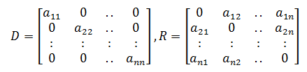
Let us decompose matrix A into a diagonal component D and remainder R such that A = D + R.
Iteratively the solution will be obtained using the below equation.
x(k+1) = D-1(b – Rx(k))
Here,
xk = kth iteration or approximation of x
x(k+1) = Next iteration of xk or (k+1)th iteration of x
The formula for the element-based method is given as

| Read more: |
Jacobian Method Formula
Given an exact approximation x(k) = (x1(k), x2(k), x3(k), …, xn(k)) for x, the procedure of Jacobian’s method helps to use the first equation and the present values of x2(k), x3(k), …, xn(k) to calculate a new value x1(k+1). Likewise, to evaluate a new value xi(k) using the ith equation and the old values of the other variables. That is, given current values x(k) = (x1(k), x2(k), …, xn(k)), determine new values by solving for x(k+1) = (x1(k+1), x2(k+1), …, xn(k+1)) in the below expression of linear equations.

The above system of equations can also be written as below.

From the above expression it is clear that, the subscript i indicates that xi(k) is the ith element of vector x(k) = (x1(k), x2(k), …, xi(k), …, xn(k) ), and superscript k corresponds to the particular iteration (not the kth power of xi ).
Assume that D, U, and L represent the diagonal, strict upper triangular and strict lower triangular and parts of matrix A, respectively, then the Jacobian’s method can be described in matrix-vector notation as given below.

This can be simplified as shown below.
Dx(k+1) + (L + U)x(k) = b
x(k+1) = D-1[(-L-U)x(k) + b]
Properties of Jacobian Method
Adding the applications of the Jacobian matrix in different areas, this method holds some important properties. The simplicity of this method is considered in both the aspects of good and bad. This method can be stated as good since it is the first iterative method and easy to understand. However, the method is also considered bad since it is not typically used in practice. Though there are cons, is still a good starting point for those who are willing to learn more useful but more complicated iterative methods.
Jacobian Method Example
Example 1:
A system of linear equations of the form Ax = b with an initial estimate x(0) is given below.

Solve the above using the Jacobian method.
Solution:
Given,

We know that x(k+1) = D-1(b – Rx(k)) is used to estimate x.
Let us rewrite the above expression in a more convenient form, i.e. D-1(b – Rx(k)) = Tx(k) + C
Here,
T = -D-1R
C = D-1b
R = L + U
Let us split matrix A as a diagonal matrix and remainder.

Upper and lower parts of reminder of A:

Here,
R = Remainder matrix
L = Lower part of R
U = Upper part of R
T = -D-1(L + U) = D-1[-L + (-U)]


Repeat the above process until it converges, i.e. until the value of ||Axn – b|| is small.
Example 2:
Solve the following system of linear equations using iterative Jacobi method.
4x1 + 2x2 – 2x3 = 0
x1 – 3x2 – x3 = 7
3x1 – x2 + 4x3 = 5
Solution:
Given,
4x1 + 2x2 – 2x3 = 0
x1 – 3x2 – x3 = 7
3x1 – x2 + 4x3 = 5
Let us write the equations to get the values of x1, x2, x3.
x1 = (1/4)[0 – 2x2 + 2x3] = (-1/2)x2 + (1/2)x3
x2 = (-1/3) [7 – (-3)x1 – (-1)x3] = (-7/3)- x1 – (1/3)x3
x3 = (1/4)[5 – 3x1 – (-x2)] = (5/4) – (3/4)x1 + (1/4)x2
Now, make the initial guess x1 = 0, x2 = 0, x3 = 0.
So, x1(1) = (-1/2)(0) + (1/2)(0) = 0
x2(1) = (-7/3)- 0 – (1/3)(0) = -7/3 = -2.333
x3(1) = (5/4) – (3/4)(0) + (1/4)(0) = 5/4 = 1.25
We can continue this iterations for the values k = 0, 1, 2,3,….
| x | k = 0 | k = 1 | k = 2 | k = 3 |
| x1(k) | 0 | 0 | 1.7917 | 1.7083 |
| x2(k) | 0 | -2.333 | -2.75 | -1.9583 |
| x3(k) | 0 | 1.25 | 0.6667 | -0.7812 |
To learn more methods of solving a system of linear equations, download BYJU’S – The Learning App.
Comments