Grouping of data plays a significant role when we have to deal with large data. This information can also be displayed using a pictograph or a bar graph. Data formed by arranging individual observations of a variable into groups, so that a frequency distribution table of these groups provides a convenient way of summarizing or analyzing the data is termed as grouped data.
Frequency distribution table for grouped data
When the collected data is large, then we can follow the below approach to analyse it easily using tally marks.
Example:
Consider the marks of 50 students of class VII obtained in an examination. The maximum marks of the exam are 50.
23, 8, 13, 18, 32, 44, 19, 8, 25, 27, 10, 30, 22, 40, 39, 17, 25, 9, 15, 20, 30, 24, 29, 19, 16, 33, 38, 46, 43, 22, 37, 27, 17, 11, 34, 41, 35, 45, 31, 26, 42, 18, 28, 30, 22, 20, 33, 39, 40, 32
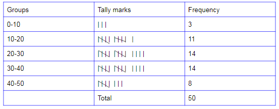
If we create a frequency distribution table for each and every observation, then it will form a large table. So for easy understanding, we can make a table with a group of observations say 0 to 10, 10 to 20 etc.

The distribution obtained in the above table is known as the grouped frequency distribution. This helps us to bring various significant inferences like:
(i) Many students have secured between 20-40, i.e. 20-30 and 30-40.
(ii) 8 students have secured higher than 40 marks, i.e. they got more than 80% in the examination.
In the above-obtained table, the groups 0-10, 10-20, 20-30,… are known as class intervals (or classes). It is observed that 10 appears in both intervals, such as 0-10 and 10-20. Similarly, 20 appears in both the intervals, such as as10-20 and 20-30. But it is not feasible that observation either 10 or 20 can belong to two classes concurrently. To avoid this inconsistency, we choose the rule that the general conclusion will belong to the higher class. It means that 10 belongs to the class interval 10-20 but not to 0-10. Similarly, 20 belongs to 20-30 but not to 10-20, etc.
Consider a class say 10-20, where 10 is the lower class interval and 20 is the upper-class interval. The difference between upper and lower class limits is called class height or class size or class width of the class interval.
Read more:
Important Questions Class 8 Maths Chapter 5 Data Handling
How to determine the class size?
In order to avoid confusion on the size of the class intervals that we need to take while grouping the data, one must follow the below steps.
Step 1: Identify the highest and the lowest (least) data values in the given observations.
Step 2: Find the difference between the highest and least value.
Step 3: Now, assume the number of class intervals we need (usually 5 to 20 classes are suggested to take based the number of observations).
Step 4: Divide the difference of highest and least value by the number of classes, this result in the size of the class interval.
Step 5: In case of any decimal number obtained as a class size take the nearest whole number greater than the obtained decimal as the class size.
Histogram
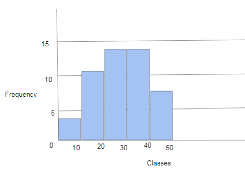
We can show the above frequency distribution table graphically using a histogram. Consider class intervals on the horizontal axis and the frequency on the vertical axis.

The height of the bars represents the frequency of the class interval. There is no gap between the bars since there is no gap between the classes.
Frequently Asked Questions – FAQs
What is grouped data and ungrouped data?
What is grouped data example?
What are the advantages of grouping data?
Assist us in concentrating on essential subgroups mainly and overlooks trivial ones
Helps in increasing the efficiency and correctness of the required estimation
Comments