Equipotential Surface

What Is Equipotential Surface?

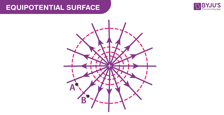
The surface, the locus of all points at the same potential, is known as the equipotential surface. No work is required to move a charge from one point to another on the equipotential surface. In other words, any surface with the same electric potential at every point is termed as an equipotential surface.

Equipotential Points: If the points in an electric field are all at the same electric potential, they are known as the equipotential points. If these points are connected by a line or a curve, it is known as an equipotential line. If such points lie on a surface, it is called an equipotential surface. Further, if these points are distributed throughout a space or a volume, it is known as an equipotential volume.

Work Done in Equipotential Surface

The work done in moving a charge between two points in an equipotential surface is zero. If a point charge is moved from point V_A to V_B in an equipotential surface, then the work done in moving the charge is given by

W = q₀(V_A –V_B)

As V_A – V_B is equal to zero, the total work done is W = 0.

Properties of Equipotential Surface

1. The electric field is always perpendicular to an equipotential surface.
2. Two equipotential surfaces can never intersect.
3. For a point charge, the equipotential surfaces are concentric spherical shells.
4. For a uniform electric field, the equipotential surfaces are planes normal to the x-axis.
5. The direction of the equipotential surface is from high potential to low potential.
6. Inside a hollow-charged spherical conductor, the potential is constant. This can be treated as equipotential volume. No work is required to move a charge from the centre to the surface.
7. For an isolated point charge, the equipotential surface is a sphere, i.e. concentric spheres around the point charge are different equipotential surfaces.
8. In a uniform electric field, any plane normal to the field direction is an equipotential surface.
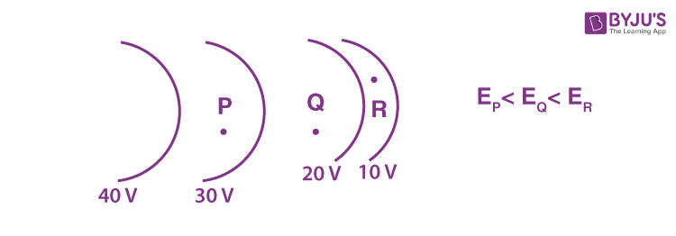
9. The spacing between equipotential surfaces enables us to identify regions of a strong and weak field, i.e., E= −dV/dr ⇒ E ∝ 1/dr.

Also Read

• Electrostatics
• Electric Charge
• Gauss Law
• Coulombs law
• Electric Field Intensity
• Electric Potential Energy
• Motion of Charged Particle in Electric Field

Problems on Equipotential Surface

Q.1: A charged particle (q =1.4 mC) moves a distance of 0.4 m along an equipotential surface of 10 V. Calculate the work done by the field during this motion.

Solution:

The work done by the field is given by the expression

W = -qΔV

Since ΔV = 0, for equipotential surfaces, the work done is zero, W = 0.

Q.2: A positive particle of charge 1.0 C accelerates in a uniform electric field of 100 V/m. The particle started from rest on an equipotential plane of 50 V. After t = 0.0002 seconds, the particle is on an equipotential plane of V = 10 volts. Determine the distance travelled by the particle.

Solution:

The work done in moving a charge in an equipotential surface is given by

W = -qΔV

Substituting the values, we get

W = (-1.0, C) (10V – 50V) = 40 J

We know that the work done in moving a charge in an electric field:

W = qEd

40 = (1.0) (100)d

d = 0.4m

Q.3: An electron of mass (m) and charge (e) is released from rest in a uniform electric field of 10⁶ newton/coulomb. Compute its acceleration. Also, find the time taken by the electron to attain a speed of 0.1 c, where c is the velocity of light. (m = 9.1 × 10^–31 kg, e = 1.6 × 10^–19 coulomb and c = 3 ×10⁸ metre/sec).

Sol.

The force experienced by the electron is

F = Ee = 10⁶ (1.6 × 10^–19)

= 1.6 × 10^–13 newton

The acceleration of the electron is given by

= 1.8 × 10¹⁷ m/sec²

The initial velocity = zero.

Let t be the time taken by the electron to attain a final speed of 0.1 c.

Now v = u + at or v = at

= 1.7 × 10¹⁰ sec.

Q.4: A ball of mass m with a charge q can rotate in a vertical plane at the end of a string of length λ in a uniform electrostatic field whose lines of force are directed upwards. What horizontal velocity must be imparted to the ball in the upper position so that the tension in the string in the lower position of the ball is 15 times the weight of the ball?

Sol.

The situation is shown in the figure.

Here, the sum of kinetic energy and potential energy at B is the same as the sum of kinetic energy and potential energy at A, i.e.,

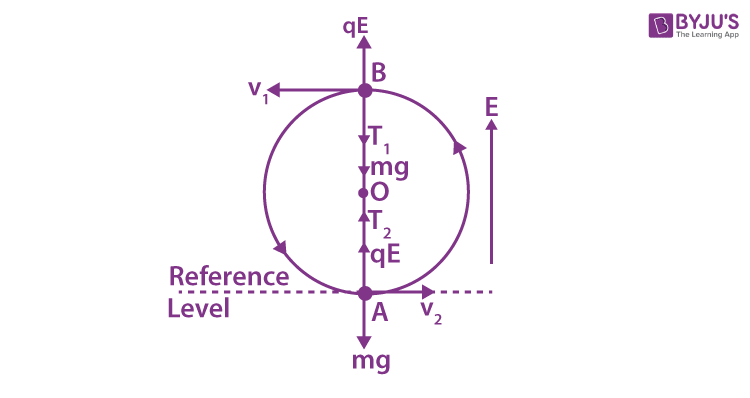
(K.E.)_B + (P.E.)_B = (K.E.)_A + (P.E.)_A ..(1)

Gain in K.E.

= (K.E.)_A – (K.E.)_B = (1/2) m (v₂² – v₁²) …(2)

Loss in P.E. = (P.E.)_B – (P.E.)_A

= Loss in gravitational P.E. – gain in electrostatic P.E.

= mg . 2λ – qE. 2λ

= (mg – qE) 2λ …(3)

From eq. (1),

(P.E.)_B – (P.E.)_A = (K.E.)_A – (K.E.)_B

Substituting the values, we get

(mg – qE) 2λ = 1/2 m (v₂² – v₁²) …(4)

Centripetal force at A = T₂ + qE – mg

From eq. (4) mv₂² = 2 (mg – qE) 2λ + mv₁²

From eq. (5) mv₂² = λ (T₂ + qE – mg)

∴ 2(mg – qE) 2λ – mv₁² = λ (T₂ + qE – mg)

or 

Putting T₂ = 15 mg, we have

Q.5: An infinite number of charges, each equal to q, are placed along the x-axis at x = 1, x = 2, x = 4, x = 8 …… and so on. Find the potential and the electric field at point x = 0 due to this set of charges.

Sol. As potential V and intensity E due to a point charge at position x are respectively given by,

And electric interaction is a two-body interaction, i.e., the principle of superposition holds good –

i.e.,

i.e.,

Q.6: On a thin rod of length λ = 1 m, lying along the x-axis with one end at the origin x = 0, there is a uniformly distributed charge per unit length λ = K_x, where K = constant = 10^–9 cm^–2. Find the work done in displacing a charge q = 1000 μC from a point (0, √(0.44) m) to (0, 1 m).

Sol.

The situation is shown in the figure. Consider a small element of length dx of the rod at a distance x from the origin. Then, potential dVP at point P due to this element is given by

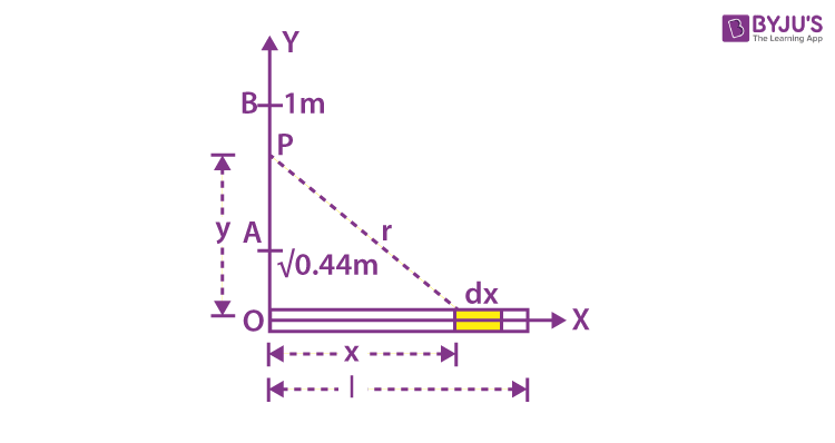
From the figure,

r² = x² + y²

or 2 r dr = 2x dx (y = constant)

On integrating this expression, we get the potential at point P. Thus,

= (9 × 10⁹) × 10^–9 × 0.5366 = 4.83 V

= (9 × 10⁹) × 10^–9× 0.4142 = 3.728 V

Net work done

= q (V_B – V_A) = 1000 × 10^–6 [3.728 – 4.83] = – 1.1 × 10^–3 Joule.

You might also be interested in the following:

• HC Verma Solutions
• HC Verma Solutions Part 1
• HC Verma Solutions Part 2