According to the CBSE Syllabus 2023-24, this chapter has been renumbered as Chapter 13.
CBSE Class 10 Maths Statistics Notes:-Download PDF Here
The brief notes on statistics for Class 10 are given here. In this, we are going to discuss important statistical concepts, such as grouped data, ungrouped data and the measures of central tendencies like mean, median and mode, methods to find the mean, median and mode, and the relationship between them with more examples.
To access the complete solutions for Class 10 Maths statistics, click on the below link.
Video Lesson on Statistics Class 10

Introduction to Statistics
Ungrouped Data
Ungrouped data is data in its original or raw form. The observations are not classified into groups.
For example, the ages of everyone present in a classroom of kindergarten kids with the teacher are as follows:
3, 3, 4, 3, 5, 4, 3, 3, 4, 3, 3, 3, 3, 4, 3, 27.
This data shows that there is one grown-up person present in this class, and that is the teacher. Ungrouped data is easy to work with when the data set is small.
Grouped Data
In grouped data, observations are organized in groups.
For example, a class of students got different marks in a school exam. The data is tabulated as follows:
| Mark interval | 0-20 | 21-40 | 41-60 | 61-80 | 81-100 |
| No. of Students | 13 | 9 | 36 | 32 | 10 |
This shows how many students got the particular mark range. Grouped data is easier to work with when a large amount of data is present.
Frequency
Frequency is the number of times a particular observation occurs in data.
For example, if four students have scored marks between 90 and 100, then the marks scored between 90 and 100 have a frequency of 4.
Class Interval
Data can be grouped into class intervals such that all observations in that range belong to that class.
Class width = upper class limit – lower class limit
Example: Consider a class interval 31 – 40.
Here, the lower class limit is 31, and the upper class limit is 40.
Hence, the size/width of the class interval 31 – 40 is calculated as follows:
Class interval size = Upper class limit – Lower class limit
Class interval size = 40 – 31 = 9
Therefore, the size of the class interval is 9.
To know more about Statistics, visit here.
Mean
Finding the mean for grouped data when class intervals are not given
If x1, x2,. . ., xn are the given observations and their respective frequencies are f1, f2, . . ., fn respectively, then the mean of the grouped data (without class interval) is given as:
For example, the marks scored by the 30 students of class 10 are given below:
| Marks obtained (xi) | 10 | 20 | 36 | 40 | 50 | 56 | 60 | 70 | 72 | 80 | 88 | 92 | 95 |
| No. of students | 1 | 1 | 3 | 4 | 3 | 2 | 4 | 4 | 1 | 1 | 2 | 3 | 1 |
We know the formula to find the mean of the grouped data is
| Marks scored (xi) | No. of students (fi) | xifi |
| 10 | 1 | 10 |
| 20 | 1 | 20 |
| 36 | 3 | 108 |
| 40 | 4 | 160 |
| 50 | 3 | 150 |
| 56 | 2 | 112 |
| 60 | 4 | 240 |
| 70 | 4 | 280 |
| 72 | 1 | 72 |
| 80 | 1 | 80 |
| 88 | 2 | 176 |
| 92 | 3 | 276 |
| 95 | 1 | 95 |
| Sum | Σfi = 30 | Σxifi = 1779 |
Now, substitute the obtained values in the formula. We get
Mean = 1779/30
Mean = 59.3
Therefore, the mean of the marks scored by the students is 59.3
Finding the mean for grouped data when class intervals are given
If x1, x2,. . ., xn is the set of observations and their frequencies are f1, f2, . . ., fn respectively, then the mean of the grouped data (with class interval) is given as follows:
Where fi is the frequency of ith class whose class mark is xi
And, “i” varies from 1 to n.
Note: Class mark =(Upper Class Limit+ Lower Class Limit)/2
Example:
Find the mean of the following grouped data:
| Class interval | 10 – 25 | 25 – 40 | 40 – 55 | 55 – 70 | 70 – 85 | 85 – 100 |
| No. of students | 2 | 3 | 7 | 6 | 6 | 6 |
To find the mean for the grouped data, first we have to find the class mark:
The formula to find the class mark is:
Class mark = (Upper class limit + Lower Class limit)/2
| Class Interval | No.of Students (fi) | Class Mark (xi) | fixi |
| 10 – 25 | 2 | 17.5 | 35.0 |
| 25 – 40 | 3 | 32.5 | 97.5 |
| 40 – 55 | 7 | 47.5 | 332.5 |
| 55 – 70 | 6 | 62.5 | 375.0 |
| 70 – 85 | 6 | 77.5 | 465.0 |
| 85 – 100 | 6 | 92.5 | 555.0 |
| Sum | Σfi = 30 | Σfixi = 1860.0 |
Now, substitute the obtained values in the mean formula, we get
Mean = 1860 / 30
Mean = 62
Therefore, the mean of the given data is 62.
Direct Method to Find Mean
Step 1: Classify the data into intervals and find the corresponding frequency of each class.
Step 2: Find the class mark by taking the midpoint of the upper and lower class limits.
Step 3: Tabulate the product of the class mark and its corresponding frequency for each class. Calculate their sum (∑xifi).
Step 4: Divide the above sum by the sum of frequencies (∑fi) to get the mean.
The formula to find the mean using the direct method is:
[Note: Find the class mark (xi) from the class interval and multiply xi by the fi (frequency)]
Assumed Mean Method to Find Mean
Step 1: Classify the data into intervals and find the corresponding frequency of each class.
Step 2: Find the class mark by taking the midpoint of the upper and lower class limits.
Step 3: Take one of the xi’s (usually one in the middle) as the assumed mean and denote it by ′a′.
Step 4: Find the deviation of ′a′ from each of the x′is
di=xi−a
Step 5: Find the mean of the deviations
Step 6: Calculate the mean as
For example, let us consider the same example as provided above.
In this method, first, we have to choose the assumed mean (a), which lies in the centre of x1, x2, …xn. Here, we choose a = 47.5.
Secondly, we have to find the difference(di), which is obtained using the formula,
di = xi – a
Now, let us see how to find the mean for the given data using the assumed mean method.
| Class Interval | No.of Students (fi) | Class Mark (xi) | di = xi – a | fidi |
| 10 – 25 | 2 | 17.5 | -30 | -60 |
| 25 – 40 | 3 | 32.5 | -15 | -45 |
| 40 – 55 | 7 | 47.5 | 0 | 0 |
| 55 – 70 | 6 | 62.5 | 15 | 90 |
| 70 – 85 | 6 | 77.5 | 30 | 180 |
| 85 – 100 | 6 | 92.5 | 45 | 270 |
| Sum | Σfi = 30 | Σfidi = 435 |
Now, using the assumed mean method formula, we can get
Mean = 47.5 + (435/30)
Mean = 47.5 + 14.5
Mean = 62
Thus, the mean of the given data using the assumed mean method is 62.
To know more about Mean, visit here.
The Relation Between the Mean of Deviations and Mean
di=xi−a
Summing over all x′is,
∑di=∑xi−∑a
Dividing throughout by ∑fi=n, Where ′n′ is the total number of observations.
For more information on The Relation between Mean of Deviations and Mean, watch the below video

To know more about Mean Deviation Formula, visit here.
Step-Deviation Method to Find Mean
Step 1: Classify the data into intervals and find the corresponding frequency of each class.
Step 2: Find the class mark by taking the midpoint of the upper and lower class limits.
Step 3: Take one of the x′is (usually one in the middle) as the assumed mean and denote it by ′a′.
Step 4: Find the deviation of a from each of the x′is
di=xi−a
Step 5: Divide all deviations −di by the class width (h) to get u′is.
Step 6: Find the mean of u′is
Step 7: Calculate the mean as
Considering the same grouped data with class interval, now let us discuss how to find the mean using the step deviation method.
Using the formula ui = (xi – a)/h
Here, a = 47.5, which is the assumed mean
Class size, h = 15.
| Class Interval | No.of Students (fi) | Class Mark (xi) | di = xi – a | ui = (xi – a)/h | fiui |
| 10 – 25 | 2 | 17.5 | -30 | -2 | -4 |
| 25 – 40 | 3 | 32.5 | -15 | -1 | -3 |
| 40 – 55 | 7 | 47.5 | 0 | 0 | 0 |
| 55 – 70 | 6 | 62.5 | 15 | 1 | 6 |
| 70 – 85 | 6 | 77.5 | 30 | 2 | 12 |
| 85 – 100 | 6 | 92.5 | 45 | 3 | 18 |
| Sum | Σfi = 30 | Σfiui = 29 |
Now, substituting the obtained values in the formula, we get
Mean = 47.5 + (15)(29/30)
Mean = 47.5 + (15)(0.967)
Mean = 47.5 + 14.5
Mean = 62
Relation Between Mean of Step- Deviations (u) and Mean
Important Relations Between Methods of Finding Mean
- All three methods of finding mean yield the same result.
- Step deviation method is easier to apply if all the deviations have a common factor.
- Assumed mean method and step deviation method are simplified versions of the direct method.
Median
Finding the median of grouped data when class intervals are not given
Step 1: Tabulate the observations and the corresponding frequency in ascending or descending order.
Step 2: Add the cumulative frequency column to the table by finding the cumulative frequency up to each observation.
Step 3: If the number of observations is odd, the median is the observation whose cumulative frequency is just greater than or equal to (n+1)/2
If the number of observations is even, the median is the average of observations whose cumulative frequency is just greater than or equal to n/2 and (n/2)+1.
The marks scored by 100 students out of 50 marks are given below. Find the median of the given data:
| Marks scored | 20 | 29 | 28 | 33 | 42 | 38 | 43 | 25 |
| No.of students | 6 | 28 | 24 | 15 | 2 | 4 | 1 | 20 |
Now, arrange the marks scored by students in ascending order.
| Marks Scored | No. of students |
| 20 | 6 |
| 25 | 20 |
| 28 | 24 |
| 29 | 28 |
| 33 | 15 |
| 38 | 4 |
| 42 | 2 |
| 43 | 1 |
| Sum | 100 |
Since the number of observations is 100, the average of the 50th and 51st observations is the median of the given data.
To find the value of the 50th and 51st observations, we have to construct the frequency table with a cumulative frequency column.
| Marks Scored | No. of students | Cumulative frequency |
| 20 | 6 | 6 |
| 25 | 20 | 26 |
| 28 | 24 | 50 |
| 29 | 28 | 78 |
| 33 | 15 | 93 |
| 38 | 4 | 97 |
| 42 | 2 | 99 |
| 43 | 1 | 100 |
From the above-given table, we can observe that,
50th observation = 28 and hence 51st observation = 29
Therefore, Median = (28 + 29)/2
Median = 57/2
Median = 28.5
Therefore, the median of the given data is 28.5.
For more information on Median, watch the below video
To know more about Median, visit here.
Cumulative Frequency
Cumulative frequency is obtained by adding all the frequencies up to a certain point.
Finding the median for grouped data when class intervals are given
Step 1: find the cumulative frequency for all class intervals.
Step 2: the median class is the class whose cumulative frequency is greater than or nearest to n2, where n is the number of observations.
Step 3: Median = l + [(N/2 – cf)/f] × h
Where,
l = lower limit of median class,
n = number of observations,
cf = cumulative frequency of class preceding the median class,
f = frequency of median class,
h = class size (assuming class size to be equal).
To learn more examples of finding the median of grouped data when class intervals are given, click here.
Cumulative Frequency Distribution of Less Than Type
The cumulative frequency of the less than type indicates the number of observations which are less than or equal to a particular observation.
Cumulative Frequency Distribution of More Than Type
A cumulative frequency of more than type indicates the number of observations that are greater than or equal to a particular observation.
To know more about Cumulative Frequency Distribution, visit here.
Visualising Formula for Median Graphically
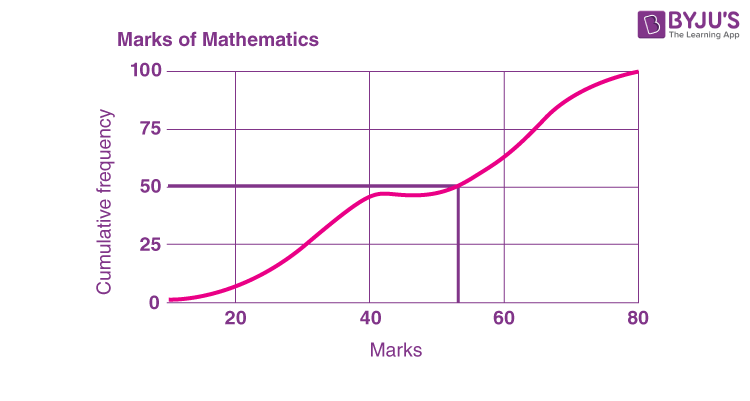
Step 1: Identify the median class.
Step 2: Mark cumulative frequencies on the y-axis and observations on the x-axis corresponding to the median class.
Step 3: Draw a straight line graph joining the extremes of class and cumulative frequencies.
Step 4: Identify the point on the graph corresponding to cf = n/2
Step 5: Drop a perpendicular from this point onto the x-axis.
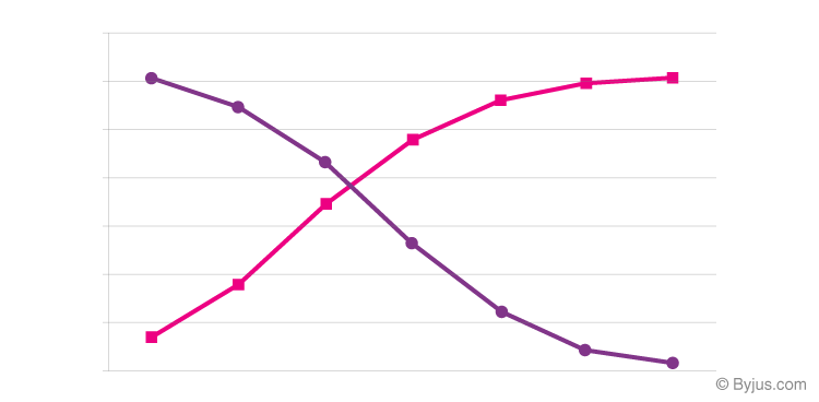
Ogive of Less Than Type
The graph of a cumulative frequency distribution of the less than type is called an ‘ogive of the less than type’.
Ogive of More Than Type
The graph of a cumulative frequency distribution of the more than type is called an ‘ogive of the more than type’.
The below diagram represents the Ogive of less than type (Rose curve) and Ogive of more than type (purple curve):
To know more about Ogive, visit here.
Relation Between the Less Than and the More Than Type Curves
The point of intersection of the ogives of more than and less than types gives the median of the grouped frequency distribution.
Mode
In statistics, the mode is the most repeated value in the given data set. In other words, the data with the highest frequency is called the mode.
For example, 4, 12, 5, 6, 5, 8, and 5 are the given set of data.
Here, the data with the highest frequency is 5, which is repeated thrice.
Therefore, the mode of the given data is 5.
Finding mode for grouped data when class intervals are not given
In grouped data without class intervals, the observation having the largest frequency is the mode.
Finding Mode for Ungrouped Data
For ungrouped data, the mode can be found out by counting the observations and using tally marks to construct a frequency table.
The observation having the largest frequency is the mode.
To get more examples of finding the mode for grouped and ungrouped data, click here.
Finding mode for grouped data when class intervals are given
For grouped data, the class having the highest frequency is called the modal class. The mode can be calculated using the following formula. The formula is valid for equal class intervals and when the modal class is unique.
Mode = l + [(f1 – f0)/(2f1 – f0 – f2)] × h
Where,
l = lower limit of modal class
h = class width
f1 = frequency of the modal class
f0 = frequency of the class preceding the modal class
f2 = frequency of the class succeeding the modal class.
To know more about Mode, visit here.
Visualising Formula for Mode Graphically
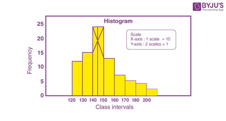
Step 1: Express the class intervals and frequencies as a histogram.
Step 2: Join the top corners of the modal class to the diagonally opposite corners of the adjacent classes
Step 3: Drop a perpendicular from the point of intersection of the above on the horizontal x-axis.
Measures of Central Tendency for Grouped Data
i) Mean is the average of a set of observations.
ii) Median is the middle value of a set of observations.
iii) A mode is the most common observation.
To know more about Central Tendency, visit here.
Empirical Relationship Between Mean, Median and Mode
i) The mean takes into account all the observations and lies between the extremes. It enables us to compare distributions.
ii) In problems where individual observations are not important, and we wish to find out a ‘typical’ observation where half the observations are below, and half the observations are above, the median is more appropriate. Median disregards extreme values.
iii) In situations that require establishing the most frequent value or most popular item, the mode is the best choice.
Mean, mode and median are connected by the empirical relationship
3 Median = Mode + 2 Mean
Solved Example
Question:
The following frequency distribution gives the monthly consumption of electricity of 68 consumers of a locality. Find the median, mean and mode of the data and compare them.
| Monthly consumption (in units) | Number of consumers |
| 65 – 85 | 4 |
| 85 – 105 | 5 |
| 105 – 125 | 13 |
| 125 – 145 | 20 |
| 145 – 165 | 14 |
| 165 – 185 | 8 |
| 185 – 205 | 4 |
Solution:
Let us find the mean of the given data.
| Class interval | Frequency (fi) | xi | di = xi – a | fidi |
| 65 – 85 | 4 | 75 | -60 | -240 |
| 85 – 105 | 5 | 95 | -40 | -200 |
| 105 – 125 | 13 | 115 | -20 | -260 |
| 125 – 145 | 20 | 135 = a | 0 | 0 |
| 145 – 165 | 14 | 155 | 20 | 280 |
| 165 – 185 | 8 | 175 | 40 | 320 |
| 185 – 205 | 4 | 195 | 60 | 240 |
| Total | ∑fi = 68 | ∑fidi = 140 |
Mean = a + (∑fidi/∑fi)
= 135 + (140/68)
= 135 + 2.05
= 137.05
Now, we need to find the cumulative frequency for the given data.
| Class interval | Frequency (fi) | Cumulative frequency |
| 65 – 85 | 4 | 4 |
| 85 – 105 | 5 | 4 + 5 = 9 |
| 105 – 125 | 13 | 9 + 13 = 22 |
| 125 – 145 | 20 | 22 + 20 = 42 |
| 145 – 165 | 14 | 42 + 14 = 56 |
| 165 – 185 | 8 | 56 + 8 = 64 |
| 185 – 205 | 4 | 64 + 4 = 68 |
N = 68
N/2 = 68/2 = 34
Cumulative frequency greater than and nearer to 34 is 42 which lies in the interval 125 – 145.
Median class: 125 – 145
Lower limit of the median class = l = 125
Frequency of the median class = f = 20
Cumulative frequency of the class preceding the median class = cf = 22
Class height = h = 20
Median = l + [(N/2 – cf)/f] × h
= 125 + [(34 – 22)/20] × 20
= 125 + 12
= 137
Let us find the mode of the given data.
Highest frequency = 20
Thus, modal class: 125 – 145
Lower limit of the modal class = l = 125
Frequency of modal class = f1 = 20
Frequency of the class preceding the modal class = f0 = 13
Frequency of the class succeeding the modal class = f2 = 14
Class height = h = 20
Mode = l + [(f1 – f0)/(2f1 – f0 – f2)] × h
= 125 + [(20 – 13)/ (2 × 20 – 13 – 14)] × 20
= 125 + [(7/(40 – 27)] × 20
= 125 + (140/13)
= 125 + 10.77
= 135.77
Therefore,
Mean = 137.05
Median = 137
Mode = 135.77
Video Lesson on Important Class 10 Statistics Questions

Practice Questions
1. The distribution below gives the weights of 30 students in a class. Find the median weight of the students and mark on Ogive curve.
| Weight (in kg) | 40 – 45 | 45 – 50 | 50 – 55 | 55 – 60 | 60 – 65 | 65 – 70 | 70 – 75 |
| Number of Students | 2 | 3 | 8 | 6 | 6 | 3 | 2 |
2. A student noted the number of cars passing through a spot on the road for 100 periods each of 3 minutes and summarised it in the table given below. Find the mode of the data.
| Number of cars | 0-10 | 10-20 | 20-30 | 30-40 | 40-50 | 50-60 | 60-70 | 70-80 |
| Frequency | 7 | 14 | 13 | 12 | 20 | 11 | 15 | 8 |
3. Consider the following distribution of daily wages of 50 workers of a factory.
| Daily wages (in Rs.) | 500 – 520 | 520 – 540 | 540 – 560 | 560 – 580 | 580 – 600 |
| Number of workers | 12 | 14 | 8 | 6 | 10 |
Find the mean daily wages of the workers of the factory by using an appropriate method.
Comments