In probability theory, the exponential distribution is defined as the probability distribution of time between events in the Poisson point process. The exponential distribution is considered as a special case of the gamma distribution. Also, the exponential distribution is the continuous analogue of the geometric distribution. In this article, we will discuss what is exponential distribution, its formula, mean, variance, memoryless property of exponential distribution, and solved examples.
Table of Contents:
- What is Exponential Distribution?
- Formula
- Mean and Variance
- Memoryless Property
- Sum of Two Independent Exponential Random Variables
- Exponential Distribution Graph
- Applications
- Example
- FAQs
What is Exponential Distribution?
In Probability theory and statistics, the exponential distribution is a continuous probability distribution that often concerns the amount of time until some specific event happens. It is a process in which events happen continuously and independently at a constant average rate. The exponential distribution has the key property of being memoryless. The exponential random variable can be either more small values or fewer larger variables. For example, the amount of money spent by the customer on one trip to the supermarket follows an exponential distribution.
Exponential Distribution Formula
The continuous random variable, say X is said to have an exponential distribution, if it has the following probability density function:
Where
λ is called the distribution rate.
Mean and Variance of Exponential Distribution
Mean:
The mean of the exponential distribution is calculated using the integration by parts.
Hence, the mean of the exponential distribution is 1/λ.
Variance:
To find the variance of the exponential distribution, we need to find the second moment of the exponential distribution, and it is given by:
Hence, the variance of the continuous random variable, X is calculated as:
Var (X) = E(X2)- E(X)2
Now, substituting the value of mean and the second moment of the exponential distribution, we get,
Thus, the variance of the exponential distribution is 1/λ2.
Memoryless Property of Exponential Distribution
The most important property of the exponential distribution is the memoryless property. This property is also applicable to the geometric distribution.
An exponentially distributed random variable “X” obeys the relation:
Pr(X >s+t |X>s) = Pr(X>t), for all s, t ≥ 0
Now, let us consider the the complementary cumulative distribution function:
= e-λt
= Pr (X>t)
Hence, Pr(X >s+t |X>s) = Pr(X>t)
This property is called the memoryless property of the exponential distribution, as we don’t need to remember when the process has started.
Sum of Two Independent Exponential Random Variables
The probability distribution function of the two independent random variables is the sum of the individual probability distribution functions.
If X1 and X2 are the two independent exponential random variables with respect to the rate parameters λ1 and λ2 respectively, then the sum of two independent exponential random variables is given by Z = X1 + X2.
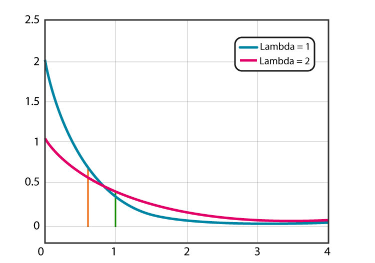
Exponential Distribution Graph
The exponential distribution graph is a graph of the probability density function which shows the distribution of distance or time taken between events. The two terms used in the exponential distribution graph is lambda (λ)and x. Here, lambda represents the events per unit time and x represents the time. The following graph shows the values for λ=1 and λ=2.
Exponential Distribution Applications
One of the widely used continuous distribution is the exponential distribution. It helps to determine the time elapsed between the events. It is used in a range of applications such as reliability theory, queuing theory, physics and so on. Some of the fields that are modelled by the exponential distribution are as follows:
- Exponential distribution helps to find the distance between mutations on a DNA strand
- Calculating the time until the radioactive particle decays.
- Helps on finding the height of different molecules in a gas at the stable temperature and pressure in a uniform gravitational field
- Helps to compute the monthly and annual highest values of regular rainfall and river outflow volumes
Exponential Distribution Problem
Example:
Assume that, you usually get 2 phone calls per hour. calculate the probability, that a phone call will come within the next hour.
Solution:
It is given that, 2 phone calls per hour. So, it would expect that one phone call at every half-an-hour. So, we can take
λ = 0.5
So, the computation is as follows:
= 0.393469
Therefore, the probability of arriving the phone calls within the next hour is 0.393469
Stay tuned with BYJU’S – The Learning App and download the app to learn with ease by exploring more Maths-related videos.
Frequently Asked Questions on Exponential Distribution
What is meant by exponential distribution?
The exponential distribution is a probability distribution function that is commonly used to measure the expected time for an event to happen.
What is the difference between the Poisson distribution and exponential distribution?
Poisson distribution deals with the number of occurrences of events in a fixed period of time, whereas the exponential distribution is a continuous probability distribution that often concerns the amount of time until some specific event happens.
What is the mean and the variance of the exponential distribution?
The mean of the exponential distribution is 1/λ and the variance of the exponential distribution is 1/λ2.
Why is the exponential distribution memoryless?
The key property of the exponential distribution is memoryless as the past has no impact on its future behaviour, and each instant is like the starting of the new random period.
What does lambda mean in the exponential distribution?
The lambda in exponential distribution represents the rate parameter, and it defines the mean number of events in an interval.