In Statistics, the probability distribution gives the possibility of each outcome of a random experiment or event. It provides the probabilities of different possible occurrences. Also read, events in probability, here.
To recall, the probability is a measure of uncertainty of various phenomena. Like, if you throw a dice, the possible outcomes of it, is defined by the probability. This distribution could be defined with any random experiments, whose outcome is not sure or could not be predicted. Let us discuss now its definition, function, formula and its types here, along with how to create a table of probability based on random variables.
| Table of Contents: |
What is Probability Distribution?
Probability distribution yields the possible outcomes for any random event. It is also defined based on the underlying sample space as a set of possible outcomes of any random experiment. These settings could be a set of real numbers or a set of vectors or a set of any entities. It is a part of probability and statistics.
Random experiments are defined as the result of an experiment, whose outcome cannot be predicted. Suppose, if we toss a coin, we cannot predict, what outcome it will appear either it will come as Head or as Tail. The possible result of a random experiment is called an outcome. And the set of outcomes is called a sample point. With the help of these experiments or events, we can always create a probability pattern table in terms of variables and probabilities.
Probability Distribution of Random Variables
A random variable has a probability distribution, which defines the probability of its unknown values. Random variables can be discrete (not constant) or continuous or both. That means it takes any of a designated finite or countable list of values, provided with a probability mass function feature of the random variable’s probability distribution or can take any numerical value in an interval or set of intervals. Through a probability density function that is representative of the random variable’s probability distribution or it can be a combination of both discrete and continuous.
Two random variables with equal probability distribution can yet vary with respect to their relationships with other random variables or whether they are independent of these. The recognition of a random variable, which means, the outcomes of randomly choosing values as per the variable’s probability distribution function, are called random variates.
Probability Distribution Formulas
| Binomial Distribution | P(X) = nCxaxbn-x
Where a = probability of success b=probability of failure n= number of trials x=random variable denoting success |
| Cumulative Distribution Function | \(\begin{array}{l}F_{X}(x)=\int_{-\infty}^{x} f_{X}(t) d t\end{array} \) |
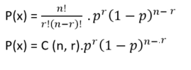
| Discrete Probability Distribution | \(\begin{array}{l}\begin{array}{l} P(x)=\frac{n !}{r !(n-r) !} \cdot p^{r}(1-p)^{n-r} \\ P(x)=C(n, r) \cdot p^{r}(1-p)^{n-r} \end{array}\end{array} \) |
Types of Probability Distribution
There are two types of probability distribution which are used for different purposes and various types of the data generation process.
-
-
- Normal or Cumulative Probability Distribution
- Binomial or Discrete Probability Distribution
-
Let us discuss now both the types along with their definition, formula and examples.
Cumulative Probability Distribution
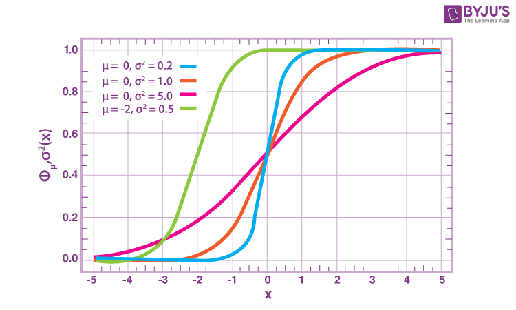
The cumulative probability distribution is also known as a continuous probability distribution. In this distribution, the set of possible outcomes can take on values in a continuous range.
For example, a set of real numbers, is a continuous or normal distribution, as it gives all the possible outcomes of real numbers. Similarly, a set of complex numbers, a set of prime numbers, a set of whole numbers etc. are examples of Normal Probability distribution. Also, in real-life scenarios, the temperature of the day is an example of continuous probability. Based on these outcomes we can create a distribution table. A probability density function describes it. The formula for the normal distribution is;
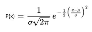
Where,
-
-
- μ = Mean Value
- σ = Standard Distribution of probability.
- If mean(μ) = 0 and standard deviation(σ) = 1, then this distribution is known to be normal distribution.
- x = Normal random variable
-
Normal Distribution Examples
Since the normal distribution statistics estimates many natural events so well, it has evolved into a standard of recommendation for many probability queries. Some of the examples are:
-
-
- Height of the Population of the world
- Rolling a dice (once or multiple times)
- To judge the Intelligent Quotient Level of children in this competitive world
- Tossing a coin
- Income distribution in countries economy among poor and rich
- The sizes of females shoes
- Weight of newly born babies range
- Average report of Students based on their performance
-
Discrete Probability Distribution
A distribution is called a discrete probability distribution, where the set of outcomes are discrete in nature.
For example, if a dice is rolled, then all the possible outcomes are discrete and give a mass of outcomes. It is also known as the probability mass function.
So, the outcomes of binomial distribution consist of n repeated trials and the outcome may or may not occur. The formula for the binomial distribution is;
Where,
-
-
- n = Total number of events
- r = Total number of successful events.
- p = Success on a single trial probability.
- nCr = [n!/r!(n−r)]!
- 1 – p = Failure Probability
-
Binomial Distribution Examples
As we already know, binomial distribution gives the possibility of a different set of outcomes. In the real-life, the concept is used for:
-
-
- To find the number of used and unused materials while manufacturing a product.
- To take a survey of positive and negative feedback from the people for anything.
- To check if a particular channel is watched by how many viewers by calculating the survey of YES/NO.
- The number of men and women working in a company.
- To count the votes for a candidate in an election and many more.
-
What is Negative Binomial Distribution?
In probability theory and statistics, if in a discrete probability distribution, the number of successes in a series of independent and identically disseminated Bernoulli trials before a particularised number of failures happens, then it is termed as the negative binomial distribution. Here the number of failures is denoted by ‘r’. For instance, if we throw a dice and determine the occurrence of 1 as a failure and all non-1’s as successes. Now, if we throw a dice frequently until 1 appears the third time, i.e.r = three failures, then the probability distribution of the number of non-1s that arrived would be the negative binomial distribution.
What is Poisson Probability Distribution?
The Poisson probability distribution is a discrete probability distribution that represents the probability of a given number of events happening in a fixed time or space if these cases occur with a known steady rate and individually of the time since the last event. It was titled after French mathematician Siméon Denis Poisson. The Poisson distribution can also be practised for the number of events happening in other particularised intervals such as distance, area or volume. Some of the real-life examples are:
-
-
- A number of patients arriving at a clinic between 10 to 11 AM.
- The number of emails received by a manager between office hours.
- The number of apples sold by a shopkeeper in the time period of 12 pm to 4 pm daily.
-
Probability Distribution Function
A function which is used to define the distribution of a probability is called a Probability distribution function. Depending upon the types, we can define these functions. Also, these functions are used in terms of probability density functions for any given random variable.
In the case of Normal distribution, the function of a real-valued random variable X is the function given by;
FX(x) = P(X ≤ x)
Where P shows the probability that the random variable X occurs on less than or equal to the value of x.
For a closed interval, (a→b), the cumulative probability function can be defined as;
P(a<X ≤ b) = FX(b) – FX(a)
If we express, the cumulative probability function as integral of its probability density function fX , then,
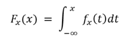
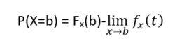
In the case of a random variable X=b, we can define cumulative probability function as;
In the case of Binomial distribution, as we know it is defined as the probability of mass or discrete random variable gives exactly some value. This distribution is also called probability mass distribution and the function associated with it is called a probability mass function.
Probability mass function is basically defined for scalar or multivariate random variables whose domain is variant or discrete. Let us discuss its formula:
Suppose a random variable X and sample space S is defined as;
X : S → A
And A ∈ R, where R is a discrete random variable.
Then the probability mass function fX : A → [0,1] for X can be defined as;
fX(x) = Pr (X=x) = P ({s ∈ S : X(s) = x})
Probability Distribution Table
The table could be created based on the random variable and possible outcomes. Say, a random variable X is a real-valued function whose domain is the sample space of a random experiment. The probability distribution P(X) of a random variable X is the system of numbers.
| X | X1 | X2 | X3 | ………….. | Xn |
| P(X) | P1 | P2 | P3 | …………… | Pn |
where Pi > 0, i=1 to n and P1+P2+P3+ …….. +Pn =1
What is the Prior Probability?
In Bayesian statistical conclusion, a prior probability distribution, also known as the prior, of an unpredictable quantity is the probability distribution, expressing one’s faiths about this quantity before any proof is taken into the record. For instance, the prior probability distribution represents the relative proportions of voters who will vote for some politician in a forthcoming election. The hidden quantity may be a parameter of the design or a possible variable rather than a perceptible variable.
What is Posterior Probability?
The posterior probability is the likelihood an event will occur after all data or background information has been brought into account. It is nearly associated with a prior probability, where an event will occur before you take any new data or evidence into consideration. It is an adjustment of prior probability. We can calculate it by using the below formula:
| Posterior Probability = Prior Probability + New Evidence |
It is commonly used in Bayesian hypothesis testing. For instance, old data propose that around 60% of students who begin college will graduate within 4 years. This is the prior probability. Still, if we think the figure is much lower, so we start collecting new data. The data collected implies that the true figure is closer to 50%, which is the posterior probability.
Solved Examples
Example 1:
A coin is tossed twice. X is the random variable of the number of heads obtained. What is the probability distribution of x?
Solution:
First write, the value of X= 0, 1 and 2, as the possibility are there that
No head comes
One head and one tail comes
And head comes in both the coins
Now the probability distribution could be written as;
P(X=0) = P(Tail+Tail) = ½ * ½ = ¼
P(X=1) = P(Head+Tail) or P(Tail+Head) = ½ * ½ + ½ *½ = ½
P(X=2) = P(Head+Head) = ½ * ½ = ¼
We can put these values in tabular form;
| X | 0 | 1 | 2 |
| P(X) | 1/4 | 1/2 | 1/4 |
Example 2:
The weight of a pot of water chosen is a continuous random variable. The following table gives the weight in kg of 100 containers recently filled by the water purifier. It records the observed values of the continuous random variable and their corresponding frequencies. Find the probability or chances for each weight category.
| Weight W | Number of Containers |
| 0.900−0.925 | 1 |
| 0.925−0.950 | 7 |
| 0.950−0.975 | 25 |
| 0.975−1.000 | 32 |
| 1.000−1.025 | 30 |
| 1.025−1.050 | 5 |
| Total | 100 |
Solution:
We first divide the number of containers in each weight category by 100 to give the probabilities.
| Weight W | Number of Containers | Probability |
| 0.900−0.925 | 1 | 0.01 |
| 0.925−0.950 | 7 | 0.07 |
| 0.950−0.975 | 25 | 0.25 |
| 0.975−1.000 | 32 | 0.32 |
| 1.000−1.025 | 30 | 0.30 |
| 1.025−1.050 | 5 | 0.05 |
| Total | 100 | 1.00 |
Related Articles
Download BYJU’S -The Learning App and get related and interactive videos to learn.
Frequently Asked Questions on Probability Distribution
What is a probability distribution in statistics?
What is an example of the probability distribution?
P(0) = ¼
P(1) = ½
P(2) = 1/4
P(x) = ¼ + ½ +¼ = 1
What is the probability distribution used for?
What is the importance of Probability distribution in Statistics?
What are the conditions of the Probability distribution?
The probabilities for random events must lie between 0 to 1.
The sum of all the probabilities of outcomes should be equal to 1.

Very useful and make my sums easily