Probability Density Function

In probability theory, a probability density function (PDF) is used to define the random variable’s probability coming within a distinct range of values, as opposed to taking on any one value. The function explains the probability density function of normal distribution and how mean and deviation exists. The standard normal distribution is used to create a database or statistics, often used in science to represent the real-valued variables whose distribution is unknown. The probability density function is explained here in this article to clear the students’ concepts in terms of their definition, properties, formulas with the help of example questions.

In this article, you will learn the probability density function definition, formula, properties, applications and how to fins the probability density function for a given function along with example.

What is the Probability Density Function?

The Probability Density Function(PDF) defines the probability function representing the density of a continuous random variable lying between a specific range of values. In other words, the probability density function produces the likelihood of values of the continuous random variable. Sometimes it is also called a probability distribution function or just a probability function. However, this function is stated in many other sources as the function over a broad set of values. Often it is referred to as cumulative distribution function or sometimes as probability mass function(PMF). However, the actual truth is PDF (probability density function ) is defined for continuous random variables, whereas PMF (probability mass function) is defined for discrete random variables.

Probability Density Function Formula

In the case of a continuous random variable, the probability taken by X on some given value x is always 0. In this case, if we find P(X = x), it does not work. Instead of this, we must calculate the probability of X lying in an interval (a, b). Now, we have to figure it for P(a< X< b), and we can calculate this using the formula of PDF. The Probability density function formula is given as,

Or

This is because, when X is continuous, we can ignore  the endpoints of intervals while finding probabilities of continuous random variables. That means, for any constants a and b,

P(a ≤ X ≤ b) = P(a < X ≤ b) = P(a ≤ X < b) = P(a < X < b).

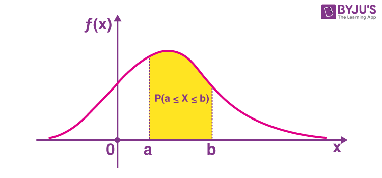
Probability Density Function Graph

The probability density function is defined as an integral of the density of the variable density over a given range. It is denoted by f (x). This function is positive or non-negative at any point of the graph, and the integral, more specifically the definite integral of PDF over the entire space is always equal to one. The graph of PDFs typically resembles a bell curve, with the probability of the outcomes below the curve. The below figure depicts the graph of a probability density function for a continuous random variable x with function f(x).

Probability Density Function Properties

Let x be the continuous random variable with density function f(x), and the probability density function should satisfy the following conditions:

• For a continuous random variable that takes some value between certain limits, say a and b, the PDF is calculated by finding the area under its curve and the X-axis within the lower limit (a) and upper limit (b). Thus, the PDF is given by
  \(\begin{array}{l}P(x)=\int_{a}^{b}f(x)\ dx\end{array} \)
• The probability density function is non-negative for all the possible values, i.e. f(x)≥ 0, for all x.
• The area between the density curve and horizontal X-axis is equal to 1, i.e.
  \(\begin{array}{l}\int_{-\infty }^{\infty}f(x)\ dx=1\end{array} \)
• Due to the property of continuous random variables, the density function curve is continued for all over the given range. Also, this defines itself over a range of continuous values or the domain of the variable.

Probability Density Function Example

Question:

Let X be a continuous random variable with the PDF given by:

Find P(0.5 < x < 1.5).

Solution:

Given PDF is:

Let us split the integral by taking the intervals as given below:

Substituting the corresponding values of f(x) based on the intervals, we get;

Integrating the functions, we get;

= [(1)²/2 – (0.5)²/2] + {[2(1.5) – (1.5)²/2] – [2(1) – (1)²/2]}

= [(½) – (⅛)] + {[3 – (9/8)] – [2 – (½)]}

= (⅜) + [(15/8) – (3/2)]

= (3 + 15 – 12)/8

= 6/8

= 3/4

Applications of Probability Density Function

PDF, i.e. the probability density function has many applications in different fields of study such as statistics, science and engineering. Some of the important applications of the probability density function are listed below:

• In Statistics, it is used to calculate the probabilities associated with the random variables.
• The probability density function is used in modelling the annual data of atmospheric NOx temporal concentration
• It is used to model the diesel engine combustion.

For more maths concepts, keep visiting BYJU’S and get various maths related videos to understand the concept in an easy and engaging way.