We already know how to plot the graph of any linear equation in two variables. The process involves plotting the points that satisfy the equation on the coordinate axis and joining them. In the problems involving linear programming, we know that we have more than one simultaneous linear equation, based on the conditions given and then we try to find the range of solutions based on the given conditions. In this article, we will try finding the solutions to Linear Programming Problems using the graphical method.
Let us try to understand this approach using an example.
The Linear Programming Problem is to maximize the profit function Z = 40x + 15y, subject to constraints,
Step-1: In the above equations, we can see that
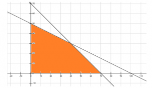
Step-2: Let us plot the linear equations x + 2y = 100 by plotting two points (0,50) and (100,0) & x + y = 70 by plotting the points (70,0) and (0,70).
Once you plot the graph with all the given constraints, the aim is to identify the Feasible Region. The feasible region is the common region that is determined by all the given constraints in the linear programming problem. In the above problem, the feasible region is shown as below:
Each and every point lying in the feasible region is the feasible choice and will satisfy all the given conditions. Any point lying outside the given feasible region is an infeasible solution and will not satisfy all the conditions simultaneously.
After potting the above graphs, we know the range of x and y that will satisfy all the given conditions. The graphical solution can also be used to find the optimal solution to the above problem. Any point in the feasible region that gives the maximum or minimum value of the objective function is called an optimal solution. In the feasible region, we can see that there are infinitely many points that satisfy the given constraints simultaneously. But how will we get the maximum or minimum value of the objective function Z = 40x + 15y?
In order to find the optimal solution, we follow the below-given theorems:
Theorem 1: Let R be the feasible region for a linear programming problem and let Z = Ax + By be the objective function. Then the optimal value (maximum or minimum) of Z will occur at a corner point (vertex) of the feasible region, provided that the optimal value of Z exists and where the variables x and y are subject to constraints described by linear inequalities.
Theorem 2: Let R be the feasible region for a linear programming problem, and let Z = Ax + By be the objective function. If R is bounded, then Z has both a maximum and a minimum value on R and each of these occurs at a corner point (vertex) of R.
If R is unbounded then the maximum and minimum value of Z may not exist, but if it exists, then it will occur at the corner point of region R.
In the above linear programming problem, the corner points are (0,0), (70,0), (40,30), and (0,50)
Substituting the above values in the objective function Z= 40x + 15y we get,
Z= 0 for (0,0)
Z= 2800 for (70,0)
Z= 2050 for (40,30)
Z= 750 for (0,50)
Hence the maximum value of Z occurs at (70,0) and the minimum value of Z occurs at (0,0).
To learn more about Graphical Method of Solving Linear Programming Problems and other related topics on linear programming, download BYJU’S – The Learning App.
very useful one