The least square method is the process of finding the best-fitting curve or line of best fit for a set of data points by reducing the sum of the squares of the offsets (residual part) of the points from the curve. During the process of finding the relation between two variables, the trend of outcomes are estimated quantitatively. This process is termed as regression analysis. The method of curve fitting is an approach to regression analysis. This method of fitting equations which approximates the curves to given raw data is the least squares.
It is quite obvious that the fitting of curves for a particular data set are not always unique. Thus, it is required to find a curve having a minimal deviation from all the measured data points. This is known as the best-fitting curve and is found by using the least-squares method.
Also, read:
Least Square Method Definition
The least-squares method is a crucial statistical method that is practised to find a regression line or a best-fit line for the given pattern. This method is described by an equation with specific parameters. The method of least squares is generously used in evaluation and regression. In regression analysis, this method is said to be a standard approach for the approximation of sets of equations having more equations than the number of unknowns.
The method of least squares actually defines the solution for the minimization of the sum of squares of deviations or the errors in the result of each equation. Find the formula for sum of squares of errors, which help to find the variation in observed data.
The least-squares method is often applied in data fitting. The best fit result is assumed to reduce the sum of squared errors or residuals which are stated to be the differences between the observed or experimental value and corresponding fitted value given in the model.
There are two basic categories of least-squares problems:
- Ordinary or linear least squares
- Nonlinear least squares
These depend upon linearity or nonlinearity of the residuals. The linear problems are often seen in regression analysis in statistics. On the other hand, the non-linear problems are generally used in the iterative method of refinement in which the model is approximated to the linear one with each iteration.
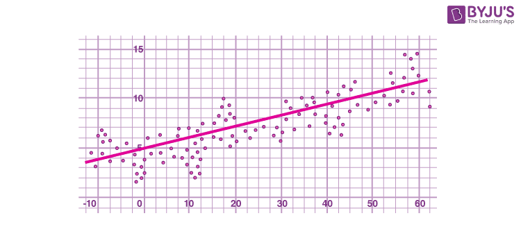
Least Square Method Graph
In linear regression, the line of best fit is a straight line as shown in the following diagram:
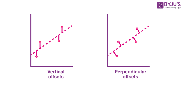
The given data points are to be minimized by the method of reducing residuals or offsets of each point from the line. The vertical offsets are generally used in surface, polynomial and hyperplane problems, while perpendicular offsets are utilized in common practice.
Least Square Method Formula
The least-square method states that the curve that best fits a given set of observations, is said to be a curve having a minimum sum of the squared residuals (or deviations or errors) from the given data points. Let us assume that the given points of data are (x1, y1), (x2, y2), (x3, y3), …, (xn, yn) in which all x’s are independent variables, while all y’s are dependent ones. Also, suppose that f(x) is the fitting curve and d represents error or deviation from each given point.
Now, we can write:
d1 = y1 − f(x1)
d2 = y2 − f(x2)
d3 = y3 − f(x3)
…..
dn = yn – f(xn)
The least-squares explain that the curve that best fits is represented by the property that the sum of squares of all the deviations from given values must be minimum, i.e:

Sum = Minimum Quantity
Suppose when we have to determine the equation of line of best fit for the given data, then we first use the following formula.
The equation of least square line is given by Y = a + bX
Normal equation for ‘a’:
∑Y = na + b∑X
Normal equation for ‘b’:
∑XY = a∑X + b∑X2
Solving these two normal equations we can get the required trend line equation.
Thus, we can get the line of best fit with formula y = ax + b
Solved Example
The Least Squares Model for a set of data (x1, y1), (x2, y2), (x3, y3), …, (xn, yn) passes through the point (xa, ya) where xa is the average of the xi‘s and ya is the average of the yi‘s. The below example explains how to find the equation of a straight line or a least square line using the least square method.
Question:
Consider the time series data given below:
| xi | 8 | 3 | 2 | 10 | 11 | 3 | 6 | 5 | 6 | 8 |
| yi | 4 | 12 | 1 | 12 | 9 | 4 | 9 | 6 | 1 | 14 |
Use the least square method to determine the equation of line of best fit for the data. Then plot the line.
Solution:
Mean of xi values = (8 + 3 + 2 + 10 + 11 + 3 + 6 + 5 + 6 + 8)/10 = 62/10 = 6.2
Mean of yi values = (4 + 12 + 1 + 12 + 9 + 4 + 9 + 6 + 1 + 14)/10 = 72/10 = 7.2
Straight line equation is y = a + bx.
The normal equations are
∑y = an + b∑x
∑xy = a∑x + b∑x2
| x | y | x2 | xy |
| 8 | 4 | 64 | 32 |
| 3 | 12 | 9 | 36 |
| 2 | 1 | 4 | 2 |
| 10 | 12 | 100 | 120 |
| 11 | 9 | 121 | 99 |
| 3 | 4 | 9 | 12 |
| 6 | 9 | 36 | 54 |
| 5 | 6 | 25 | 30 |
| 6 | 1 | 36 | 6 |
| 8 | 14 | 64 | 112 |
| ∑x = 62 | ∑y = 72 | ∑x2 = 468 | ∑xy = 503 |
Substituting these values in the normal equations,
10a + 62b = 72….(1)
62a + 468b = 503….(2)
(1) × 62 – (2) × 10,
620a + 3844b – (620a + 4680b) = 4464 – 5030
-836b = -566
b = 566/836
b = 283/418
b = 0.677
Substituting b = 0.677 in equation (1),
10a + 62(0.677) = 72
10a + 41.974 = 72
10a = 72 – 41.974
10a = 30.026
a = 30.026/10
a = 3.0026
Therefore, the equation becomes,
y = a + bx
y = 3.0026 + 0.677x
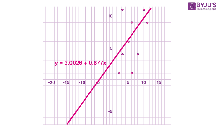
This is the required trend line equation.
Now, we can find the sum of squares of deviations from the obtained values as:
d1 = [4 – (3.0026 + 0.677*8)] = (-4.4186)
d2 = [12 – (3.0026 + 0.677*3)] = (6.9664)
d3 = [1 – (3.0026 + 0.677*2)] = (-3.3566)
d4 = [12 – (3.0026 + 0.677*10)] = (2.2274)
d5 = [9 – (3.0026 + 0.677*11)] =(-1.4496)
d6 = [4 – (3.0026 + 0.677*3)] = (-1.0336)
d7 = [9 – (3.0026 + 0.677*6)] = (1.9354)
d8 = [6 – (3.0026 + 0.677*5)] = (-0.3876)
d9 = [1 – (3.0026 + 0.677*6)] = (-6.0646)
d10 = [14 – (3.0026 + 0.677*8)] = (5.5814)
∑d2 = (-4.4186)2 + (6.9664)2 + (-3.3566)2 + (2.2274)2 + (-1.4496)2 + (-1.0336)2 + (1.9354)2 + (-0.3876)2 + (-6.0646)2 + (5.5814)2 = 159.27990
Limitations for Least-Square Method
The least-squares method is a very beneficial method of curve fitting. Despite many benefits, it has a few shortcomings too. One of the main limitations is discussed here.
In the process of regression analysis, which utilizes the least-square method for curve fitting, it is inevitably assumed that the errors in the independent variable are negligible or zero. In such cases, when independent variable errors are non-negligible, the models are subjected to measurement errors. Therefore, here, the least square method may even lead to hypothesis testing, where parameter estimates and confidence intervals are taken into consideration due to the presence of errors occurring in the independent variables.
Frequently Asked Questions – FAQs
How do you calculate least squares?
The least-squares explain that the curve that best fits is represented by the property that the sum of squares of all the deviations from given values must be minimum.
How many methods are available for the Least Square?
Ordinary or linear least squares
Nonlinear least squares
Comments