In probability theory and statistics, the Normal Distribution, also called the Gaussian Distribution, is the most significant continuous probability distribution. Sometimes it is also called a bell curve. A large number of random variables are either nearly or exactly represented by the normal distribution, in every physical science and economics. Furthermore, it can be used to approximate other probability distributions, therefore supporting the usage of the word ‘normal ‘as in about the one, mostly used.
Table of Contents:
- Definition
- Formula
- Curve
- Normal Distribution Standard Deviation
- Table
- Problems and Solutions
- Properties
- Applications
- FAQs
Normal Distribution Definition
The Normal Distribution is defined by the probability density function for a continuous random variable in a system. Let us say, f(x) is the probability density function and X is the random variable. Hence, it defines a function which is integrated between the range or interval (x to x + dx), giving the probability of random variable X, by considering the values between x and x+dx.
f(x) ≥ 0 ∀ x ϵ (−∞,+∞)
Normal Distribution Formula
The probability density function of normal or gaussian distribution is given by;

Where,
- x is the variable
- μ is the mean
- σ is the standard deviation
Also, read:
Normal Distribution Curve
The random variables following the normal distribution are those whose values can find any unknown value in a given range. For example, finding the height of the students in the school. Here, the distribution can consider any value, but it will be bounded in the range say, 0 to 6ft. This limitation is forced physically in our query.
Whereas, the normal distribution doesn’t even bother about the range. The range can also extend to –∞ to + ∞ and still we can find a smooth curve. These random variables are called Continuous Variables, and the Normal Distribution then provides here probability of the value lying in a particular range for a given experiment. Also, use the normal distribution calculator to find the probability density function by just providing the mean and standard deviation value.
Normal Distribution Standard Deviation
Generally, the normal distribution has any positive standard deviation. We know that the mean helps to determine the line of symmetry of a graph, whereas the standard deviation helps to know how far the data are spread out. If the standard deviation is smaller, the data are somewhat close to each other and the graph becomes narrower. If the standard deviation is larger, the data are dispersed more, and the graph becomes wider. The standard deviations are used to subdivide the area under the normal curve. Each subdivided section defines the percentage of data, which falls into the specific region of a graph.
Using 1 standard deviation, the Empirical Rule states that,
- Approximately 68% of the data falls within one standard deviation of the mean. (i.e., Between Mean- one Standard Deviation and Mean + one standard deviation)
- Approximately 95% of the data falls within two standard deviations of the mean. (i.e., Between Mean- two Standard Deviation and Mean + two standard deviations)
- Approximately 99.7% of the data fall within three standard deviations of the mean. (i.e., Between Mean- three Standard Deviation and Mean + three standard deviations)
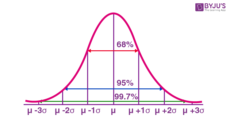
Thus, the empirical rule is also called the 68 – 95 – 99.7 rule.
Normal Distribution Table
The table here shows the area from 0 to Z-value.
| Z-Value | 0.00 | 0.01 | 0.02 | 0.03 | 0.04 | 0.05 | 0.06 | 0.07 | 0.08 | 0.09 |
| 0.0 | 0.0000 | 0.0040 | 0.0080 | 0.0120 | 0.0160 | 0.0199 | 0.0239 | 0.0279 | 0.0319 | 0.0359 |
| 0.1 | 0.0398 | 0.0438 | 0.0478 | 0.0517 | 0.0557 | 0.0596 | 0.0636 | 0.0675 | 0.0714 | 0.0753 |
| 0.2 | 0.0793 | 0.0832 | 0.0871 | 0.0910 | 0.0948 | 0.0987 | 0.1026 | 0.1064 | 0.1103 | 0.1141 |
| 0.3 | 0.1179 | 0.1217 | 0.1255 | 0.1293 | 0.1331 | 0.1368 | 0.1406 | 0.1443 | 0.1480 | 0.1517 |
| 0.4 | 0.1554 | 0.1591 | 0.1628 | 0.1664 | 0.1700 | 0.1736 | 0.1772 | 0.1808 | 0.1844 | 0.1879 |
| 0.5 | 0.1915 | 0.1950 | 0.1985 | 0.2019 | 0.2054 | 0.2088 | 0.2123 | 0.2157 | 0.2190 | 0.2224 |
| 0.6 | 0.2257 | 0.2291 | 0.2324 | 0.2357 | 0.2389 | 0.2422 | 0.2454 | 0.2486 | 0.2517 | 0.2549 |
| 0.7 | 0.2580 | 0.2611 | 0.2642 | 0.2673 | 0.2704 | 0.2734 | 0.2764 | 0.2794 | 0.2823 | 0.2852 |
| 0.8 | 0.2881 | 0.2910 | 0.2939 | 0.2967 | 0.2995 | 0.3023 | 0.3051 | 0.3078 | 0.3106 | 0.3133 |
| 0.9 | 0.3159 | 0.3186 | 0.3212 | 0.3238 | 0.3264 | 0.3289 | 0.3315 | 0.3340 | 0.3365 | 0.3389 |
| 1.0 | 0.3413 | 0.3438 | 0.3461 | 0.3485 | 0.3508 | 0.3531 | 0.3554 | 0.3577 | 0.3599 | 0.3621 |
| 1.1 | 0.3643 | 0.3665 | 0.3686 | 0.3708 | 0.3729 | 0.3749 | 0.3770 | 0.3790 | 0.3810 | 0.3830 |
| 1.2 | 0.3849 | 0.3869 | 0.3888 | 0.3907 | 0.3925 | 0.3944 | 0.3962 | 0.3980 | 0.3997 | 0.4015 |
| 1.3 | 0.4032 | 0.4049 | 0.4066 | 0.4082 | 0.4099 | 0.4115 | 0.4131 | 0.4147 | 0.4162 | 0.4177 |
| 1.4 | 0.4192 | 0.4207 | 0.4222 | 0.4236 | 0.4251 | 0.4265 | 0.4279 | 0.4292 | 0.4306 | 0.4319 |
| 1.5 | 0.4332 | 0.4345 | 0.4357 | 0.4370 | 0.4382 | 0.4394 | 0.4406 | 0.4418 | 0.4429 | 0.4441 |
| 1.6 | 0.4452 | 0.4463 | 0.4474 | 0.4484 | 0.4495 | 0.4505 | 0.4515 | 0.4525 | 0.4535 | 0.4545 |
| 1.7 | 0.4554 | 0.4564 | 0.4573 | 0.4582 | 0.4591 | 0.4599 | 0.4608 | 0.4616 | 0.4625 | 0.4633 |
| 1.8 | 0.4641 | 0.4649 | 0.4656 | 0.4664 | 0.4671 | 0.4678 | 0.4686 | 0.4693 | 0.4699 | 0.4706 |
| 1.9 | 0.4713 | 0.4719 | 0.4726 | 0.4732 | 0.4738 | 0.4744 | 0.4750 | 0.4756 | 0.4761 | 0.4767 |
| 2.0 | 0.4772 | 0.4778 | 0.4783 | 0.4788 | 0.4793 | 0.4798 | 0.4803 | 0.4808 | 0.4812 | 0.4817 |
| 2.1 | 0.4821 | 0.4826 | 0.4830 | 0.4834 | 0.4838 | 0.4842 | 0.4846 | 0.4850 | 0.4854 | 0.4857 |
| 2.2 | 0.4861 | 0.4864 | 0.4868 | 0.4871 | 0.4875 | 0.4878 | 0.4881 | 0.4884 | 0.4887 | 0.4890 |
| 2.3 | 0.4893 | 0.4896 | 0.4898 | 0.4901 | 0.4904 | 0.4906 | 0.4909 | 0.4911 | 0.4913 | 0.4916 |
| 2.4 | 0.4918 | 0.4920 | 0.4922 | 0.4925 | 0.4927 | 0.4929 | 0.4931 | 0.4932 | 0.4934 | 0.4936 |
| 2.5 | 0.4938 | 0.4940 | 0.4941 | 0.4943 | 0.4945 | 0.4946 | 0.4948 | 0.4949 | 0.4951 | 0.4952 |
| 2.6 | 0.4953 | 0.4955 | 0.4956 | 0.4957 | 0.4959 | 0.4960 | 0.4961 | 0.4962 | 0.4963 | 0.4964 |
| 2.7 | 0.4965 | 0.4966 | 0.4967 | 0.4968 | 0.4969 | 0.4970 | 0.4971 | 0.4972 | 0.4973 | 0.4974 |
| 2.8 | 0.4974 | 0.4975 | 0.4976 | 0.4977 | 0.4977 | 0.4978 | 0.4979 | 0.4979 | 0.4980 | 0.4981 |
| 2.9 | 0.4981 | 0.4982 | 0.4982 | 0.4983 | 0.4984 | 0.4984 | 0.4985 | 0.4985 | 0.4986 | 0.4986 |
| 3.0 | 0.4987 | 0.4987 | 0.4987 | 0.4988 | 0.4988 | 0.4989 | 0.4989 | 0.4989 | 0.4990 | 0.4990 |
Normal Distribution Problems and Solutions
Question 1: Calculate the probability density function of normal distribution using the following data. x = 3, μ = 4 and σ = 2.
Solution: Given, variable, x = 3
Mean = 4 and
Standard deviation = 2
By the formula of the probability density of normal distribution, we can write;

Hence, f(3,4,2) = 1.106.
Question 2: If the value of random variable is 2, mean is 5 and the standard deviation is 4, then find the probability density function of the gaussian distribution.
Solution: Given,
Variable, x = 2
Mean = 5 and
Standard deviation = 4
By the formula of the probability density of normal distribution, we can write;

f(2,2,4) = 1/(4√2π) e0
f(2,2,4) = 0.0997
There are two main parameters of normal distribution in statistics namely mean and standard deviation. The location and scale parameters of the given normal distribution can be estimated using these two parameters.
Normal Distribution Properties
Some of the important properties of the normal distribution are listed below:
- In a normal distribution, the mean, median and mode are equal.(i.e., Mean = Median= Mode).
- The total area under the curve should be equal to 1.
- The normally distributed curve should be symmetric at the centre.
- There should be exactly half of the values are to the right of the centre and exactly half of the values are to the left of the centre.
- The normal distribution should be defined by the mean and standard deviation.
- The normal distribution curve must have only one peak. (i.e., Unimodal)
- The curve approaches the x-axis, but it never touches, and it extends farther away from the mean.
Applications
The normal distributions are closely associated with many things such as:
- Marks scored on the test
- Heights of different persons
- Size of objects produced by the machine
- Blood pressure and so on.
Frequently Asked Questions on Normal Distribution – FAQs
What is a normal distribution in statistics?
What does normal distribution mean?
What is a normal distribution used for?
What are the characteristics of a normal distribution?
It is symmetric, unimodal (i.e., one mode), and asymptotic.
The values of mean, median, and mode are all equal.
A normal distribution is quite symmetrical about its center. That means the left side of the center of the peak is a mirror image of the right side. There is also only one peak (i.e., one mode) in a normal distribution.