We have seen that the total energy of a harmonic oscillator remains constant. Once started, the oscillations continue forever with a constant amplitude (which is determined from the initial conditions) and a constant frequency (which is determined by the inertial and elastic properties of the system). Simple harmonic motions which persist indefinitely without loss of amplitude are called free or undamped oscillation.
However, observation of the free oscillations of a real physical system reveals that the energy of the oscillator gradually decreases with time, and the oscillator eventually comes to rest. For example, the amplitude of a pendulum oscillating in the air decreases with time, and it ultimately stops. The vibrations of a tuning fork die away with the passage of time. This happens because, in actual physical systems, friction (or damping) is always present. Friction resists motion.
The presence of resistance to motion implies that frictional or damping force acts on the system. The damping force acts in opposition to the motion, doing negative work on the system, leading to a dissipation of energy. When a body moves through a medium such as air, water, etc., its energy is dissipated due to friction and appears as heat either in the body itself or in the surrounding medium or both.
There is another mechanism by which an oscillator loses energy. The energy of an oscillator may decrease not only due to friction in the system but also due to radiation. The oscillating body imparts periodic motion to the particles of the medium in which it oscillates, thus producing waves. For example, a tuning fork produces sound waves in the medium, which results in a decrease in its energy.
All sounding bodies are subject to dissipative forces, or otherwise, there would be no loss of energy by the body, and consequently, no emission of sound energy could occur. Thus, sound waves are produced by radiation from mechanical oscillatory systems. We will learn later that electromagnetic waves are produced by radiations from oscillating electric and magnetic fields.
The effect of radiation by an oscillating system and of the friction present in the system is that the amplitude of oscillations gradually diminishes with time. The reduction in amplitude (or energy) of an oscillator is called damping, and the oscillation is said to be damped.
Damping Forces
The damping of a real system is a complex phenomenon involving several kinds of damping forces.
- The damping force opposes the motion of the body
- The magnitude of the damping force is directly proportional to the velocity of the body
- The direction of the damping force is opposite to the velocity.
- Damping force is denoted by Fd.Fd = – pv, where v is the magnitude of the velocity of the object and p, the viscous damping coefficient, represents the damping force per unit velocity. The negative sign indicates that the force opposes the motion, tending to reduce velocity. In other words, the viscous damping force is a retarding force.
The damping force that depends on velocity is referred to as viscous damping force. Since the velocity of most oscillating systems is usually small, the damping force exerted by the fluid in contact with the system is likely to be viscous. Viscous forces are generally much smaller than inertial and elastic forces in a system.
However, damping devices, called dampers, are sometimes deliberately introduced in a system for vibration control. The damping force exerted by such devices may be comparable in magnitude to the inertial and elastic forces.
In real systems, it is likely that the moving part is in contact with an unlubricated surface, as in the case of horizontal oscillations of a body attached to a spring (see figure). The oscillating body is always in contact with the horizontal surface. The resulting frictional force opposes the motion and can often be idealised as a force of constant magnitude. Such a force is usually referred to as a Coulomb friction force.
In a solid, some part of energy may be lost due to imperfect elasticity or internal friction of the material. It is very difficult to estimate this type of damping. Experiments suggest that a resistive force proportional to the amplitude and independent of the frequency may serve as a satisfactory approximation. This kind of damping in solids is referred to as structural damping.
Thus, the damping of a real system is a complex phenomenon involving several kinds of damping forces, such as viscous damping, Coulomb friction and structural damping. Because it is generally very difficult to predict the magnitude of the damping forces, one usually has to rely on experience and experiment so as to make a reasonably good estimate. It is a common practice to approximate the damping of a system by equivalent viscous damping for the simple reason that viscous damping is the most convenient to handle mathematically. Thus, according to this approximation, the magnitude of the viscous force to be used in a particular problem is chosen to be the one that would produce the same rate of energy dissipation as the actual damping forces. This usually provides a good estimate.
The inclusion of damping forces complicates the analysis considerably. Fortunately, in actual systems, the damping forces are usually small and can often be ignored. In situations where they are not negligibly small, the viscous damping model is the most convenient mathematically. We shall use this model under the simplifying assumption that the velocity of the moving part of the system is small so that the damping force is linear in velocity.
If the velocity is not small, the damping force exerted on the system may be represented more closely by force proportional to the square of the velocity. We shall not deal with such forces. The effect of the linear viscous damping force on the free oscillations of simple systems with one degree of freedom is considered in the next section.
Damped Oscillations of a System Having One Degree of Freedom
We will investigate the effect of damping on the harmonic oscillations of a simple system having one degree of freedom. One such system is shown in the figure. When the system is displaced from its equilibrium state and released, it begins to move. The forces acting on the system are given below:
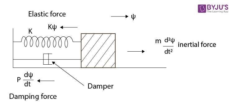
(i) A restoring force –Kx, where K is the coefficient of the restoring force, and x is the displacement
(ii) A damping force -p(dx/dt), where p is the coefficient of the damping force and (dx/dt) is the velocity of the moving part of the system. From Newton’s law for a rigid body in translation, these forces must balance with Newton’s force m(d2x/dt2), where m is the mass of the oscillator and (d2x/dt2) is its acceleration. Since the restoring force and the damping force acts in a direction opposite to Newton’s force, we have
\(\begin{array}{l}m\frac{{{d}^{2}}x}{d{{t}^{2}}}=-Kx-p\frac{dx}{dt}….(3.1)\end{array} \)
Remember, this equation holds only for small displacements and small velocities. This equation can be rewritten as:
\(\begin{array}{l}\frac{{{d}^{2}}x}{d{{t}^{2}}}+\gamma \frac{dx}{dt}+\omega _{0}^{2}x=0….(3.2)\end{array} \)
With
\(\begin{array}{l}\gamma =p/m….(3.3)\end{array} \)
And
\(\begin{array}{l}\omega _{0}^{2}=K/m….(3.4)\end{array} \)
Notice that dimensionally
\(\begin{array}{l}\gamma =\frac{p}{m}=\frac{\text{force}}{\text{velocity }\!\!\times\!\!\text{ mass}}=\frac{\text{ML}{{\text{T}}^{-2}}}{\text{L}{{\text{T}}^{-1}}M}={{T}^{-1}}.\end{array} \)
the same as the dimension of frequency.
It is easy to see that in Equation (3.2), the damping is characterised by the quantity γ, having the dimension of frequency, and the constant ω0 represents the angular frequency of the system in the absence of damping and is called the natural frequency of the oscillator. Equation (3.2) is the differential equation of the damped oscillator. To find out how the displacement varies with time, we need to solve Equation (3.2) with constants γ and ω0 given, respectively, by Equations (3.3) and (3.4).
The General Solution
To solve Equation (3.2), we make use of the exponential function again. Let us assume that the solution is
\(\begin{array}{l}x=A{{e}^{\alpha t}}\end{array} \)
And solve for α. Constants A and α are arbitrary and as yet undetermined. Differentiating, we have
\(\begin{array}{l}\frac{dx}{dt}=\alpha A\,\,{{e}^{\alpha t}}\end{array} \)
\(\begin{array}{l}\frac{{{d}^{2}}x}{d{{t}^{2}}}={{\alpha }^{2}}A\,\,{{e}^{\alpha t}}\end{array} \)
Substitution in Equation (3.2) yields
\(\begin{array}{l}\left( {{\alpha }^{2}}+\gamma \alpha +\omega _{0}^{2} \right)A\,{{e}^{\alpha t}}=0\end{array} \)
For this equation to hold for all values of t, the term in the brackets must vanish, i.e.,
\(\begin{array}{l}{{\alpha }^{2}}+\gamma \alpha +\omega _{0}^{2}=0\end{array} \)
The two roots of this quadratic equation are
\(\begin{array}{l}{{\alpha }_{1}}=-\frac{\gamma }{2}+\frac{1}{2}{{\left( {{\gamma }^{2}}-4\omega _{0}^{2} \right)}^{1/2}}\end{array} \)
And
\(\begin{array}{l}{{\alpha }_{2}}=-\frac{\gamma }{2}-\frac{1}{2}{{\left( {{\gamma }^{2}}-4\omega _{0}^{2} \right)}^{1/2}}\end{array} \)
Thus, the two possible solutions of Equation (3.2) are
\(\begin{array}{l}{{x}_{1}}={{A}_{1}}\,\,{{e}^{\alpha }}{{1}^{t}}={{A}_{1}}\,\exp \left[ -\frac{\gamma }{2}+\frac{1}{2}{{\left( {{\gamma }^{2}}-4\omega _{0}^{2} \right)}^{1/2}} \right]t\end{array} \)
And
\(\begin{array}{l}{{x}_{2}}={{A}_{2}}\,\,{{e}^{\alpha }}{{2}^{t}}={{A}_{2}}\,\exp \left[ -\frac{\gamma }{2}-\frac{1}{2}{{\left( {{\gamma }^{2}}-4\omega _{0}^{2} \right)}^{1/2}} \right]t\end{array} \)
Since Equation (3.2) is linear, the superposition principle is applicable. Hence, the general solution is given by the superposition of the two solutions, i.e.,
\(\begin{array}{l}x={{x}_{1}}+{{x}_{2}}\end{array} \)
Or
\(\begin{array}{l}x={{A}_{1}}\,\exp \left[ -\frac{\gamma }{2}+{{\left( \frac{{{\gamma }^{2}}}{4}-\omega _{0}^{2} \right)}^{1/2}} \right]t +{{A}_{2}}\,\exp \left[ -\frac{\gamma }{2}-{{\left( \frac{{{\gamma }^{2}}}{4}-\omega _{0}^{2} \right)}^{1/2}} \right]t….(3.5)\end{array} \)
Here A1 and A2 are arbitrary constants to be determined from the initial conditions, namely, the initial displacement and the initial velocity.
The nature of the motion depends on the character of the roots α1 and α2. The roots may be real or complex, depending on whether γ > 2ω0 or γ < 2ω0 and γ < 2 ω0. Each condition describes a particular kind of behaviour of the system. We shall now treat each case separately.
Case I:
γ > 2 ω0 (Large Damping) In this case, the damping term γ/2 dominates the stiffness term ω0 and the term
\(\begin{array}{l}{{\left( {{\gamma }^{2}}/4-\omega _{0}^{2} \right)}^{1/2}}\end{array} \)
in Eq. (3.5) is a real quantity with a positive value, say, q, i.e.,
\(\begin{array}{l}{{\left( \frac{{{\gamma }^{2}}}{4}-\omega _{0}^{2} \right)}^{1/2}}=q\end{array} \)
So that displacement ψ as a function of time is given by
\(\begin{array}{l}x={{A}_{1}}\,\exp \left( -\frac{\gamma }{2}+q \right)t+{{A}_{2}}\,\exp \left( -\frac{\gamma }{2}+q \right)t….(3.6)\end{array} \)
The velocity is given by
\(\begin{array}{l}\frac{dx}{dt}=\left( -\frac{\gamma }{2}+q \right){{A}_{1}}\,\exp \left( -\frac{\gamma }{2}+q \right)t -\left( \frac{\gamma }{2}+q \right){{A}_{2}}\,\exp \left( -\frac{\gamma }{2}+q \right)t….(3.7)\end{array} \)
These equations describe the behaviour of a heavily damped oscillator, for example, a pendulum in a viscous medium such as a dense oil. As stated earlier, the constants A1 and A2 are determined from the initial conditions. Let us assume that the oscillator is at its equilibrium position) (ψ = 0) at time t = 0. At this instant, it is given a kick so that it has a finite velocity, say, V0 at this time, i.e., at t = 0.
x = 0
Equations (3.6) and (3.7) then give (setting t = 0)
\(\begin{array}{l}0={{A}_{1}}+{{A}_{2}}\end{array} \)
\(\begin{array}{l}{{V}_{0}}=\left( -\frac{\gamma }{2}+q \right){{A}_{1}}-\left( \frac{\gamma }{2}+q \right){{A}_{2}}\end{array} \)
giving
\(\begin{array}{l}{{A}_{1}}=-{{A}_{2}}=\frac{{{V}_{0}}}{2q}\end{array} \)
Thus, under the above initial conditions, Equations (3.6) and (3.7) become
\(\begin{array}{l}x=\frac{{{V}_{0}}}{2q}{{e}^{-\gamma t/2}}\left( {{e}^{qt}}-{{e}^{-qt}} \right)\end{array} \)
Or
\(\begin{array}{l}x=\frac{{{V}_{0}}}{q}{{e}^{-\gamma t/2}}\sinh \left( qt \right)\end{array} \)
And
\(\begin{array}{l}\frac{dx}{dt}=\frac{{{V}_{0}}}{2}{{e}^{-\gamma t/2}}\left\{ \left( {{e}^{qt}}+{{e}^{-qt}} \right)-\frac{\gamma }{2q}\left( {{e}^{qt}}-{{e}^{-qt}} \right) \right\}\end{array} \)
Or
\(\begin{array}{l}\frac{dx}{dt}={{V}_{0}}{{e}^{-\gamma t/2}}\left\{ \cosh \left( qt \right)-\frac{\gamma }{2q}\sinh \left( qt \right) \right\}….(3.9)\end{array} \)
Figure 1 illustrates the behaviour of a heavily damped system when it is disturbed from equilibrium by a sudden impulse at t = 0. It is the displacement – time graph of Equation (3.8). For small values of time t, the term
\(\begin{array}{l}{{e}^{-\gamma t/2}}\end{array} \)
is very nearly unity; the displacement increases with time since sinh (qt) increases as t increases. Very soon, however, the term \(\begin{array}{l}{{e}^{-\gamma t/2}}\end{array} \)
starts contributing, and the displacement decays exponentially with time, eventually becoming zero. The turning point occurs at a time \(\begin{array}{l}t={{t}_{0}}\end{array} \)
when \(\begin{array}{l}dx/dt=0.\end{array} \)
Equation (3.9) tells us that this happens at a time t = to, satisfying
\(\begin{array}{l}\tan \,h\left( q{{t}_{0}} \right)=\frac{2q}{\gamma }\end{array} \)
Thus, the displacement increases until the time
\(\begin{array}{l}t={{t}_{0}},\end{array} \)
, after which it slowly returns to zero. Since displacement ψ never becomes negative, there is no oscillation at all. Such a motion is called deadbeat. We come across such a motion in the case of a deadbeat galvanometer (see sec. 3.6).
Case II:
\(\begin{array}{l}\gamma =2\,{{\omega }_{0}}\end{array} \)
(Critical Damping). This is a special case of a heavily damped motion. Using the notation \(\begin{array}{l}q={{\left( {{\gamma }^{2}}/4-\omega _{0}^{2} \right)}^{t/2}}\end{array} \)
of case I, we see that, in this case, q = 0 and Eq. (3.6) becomes
\(\begin{array}{l}x=\left( {{A}_{1}}+{{A}_{2}} \right){{e}^{-\gamma t/2}}\end{array} \)
Or
\(\begin{array}{l}x=B\,{{e}^{-\gamma t/2}}….(3.10)\end{array} \)
Where, B = A1 + A2 is a constant. In other words, Equation (3.10) is the solution of Equation (3.2) for γ = 2 ω0. In this case, the two roots α1 and α2 become identical. Notice that the solution (3.10) contains only one adjustable constant, B. This solution is only a partial solution since the solution of any second-order differential equation must contain two adjustable constants. This can be understood as follows. If Equation (3.10) was a complete solution of Equation (3.2), then the velocity of the oscillator would be given by
\(\begin{array}{l}\frac{dx}{dt}=-B\frac{\gamma }{2}{{e}^{-\gamma t/2}}\end{array} \)
When the system is disturbed from equilibrium (x = 0) by giving an impulse (i.e., by imparting a velocity V0) at t = 0, we have, from the above two equations,
B = 0
\(\begin{array}{l}{{V}_{0}}=-\frac{\gamma }{2}B\end{array} \)
Implying, thereby, that V0 is also zero, which is not our initial condition. Hence, our trial solution yields only a partial solution in the case when q = 0.
We can verify that a second solution is represented by the trial solution
\(\begin{array}{l}x=Ct\,{{e}^{-\gamma t/2}}\end{array} \)
Giving
\(\begin{array}{l}\frac{dx}{dt}=C\,{{e}^{-\gamma t/2}}\left( 1-\frac{\gamma t}{2} \right)\end{array} \)
And
\(\begin{array}{l}\frac{{{d}^{2}}x}{d{{t}^{2}}}=C\,\frac{\gamma }{2}{{e}^{-\gamma t/2}}\left( -2+\frac{\gamma t}{2} \right)\end{array} \)
Substituting for x,
\(\begin{array}{l}\frac{dx}{dt}\,and\,\,\frac{d{{x}^{2}}}{d{{t}^{2}}}\end{array} \)
in Eq. (3.2) with ωo2 replaced by \(\begin{array}{l}\frac{{{\gamma }^{2}}}{4}\end{array} \)
i.e.
\(\begin{array}{l}\frac{{{d}^{2}}x}{d{{t}^{2}}}+\gamma \frac{dx}{dt}+\frac{{{\gamma }^{2}}}{4}x=0\end{array} \)
We have,
\(\begin{array}{l}C\frac{\gamma }{2}{{e}^{-\gamma t/2}}\left( -2+\frac{\gamma t}{2} \right)+\gamma C\,{{e}^{-\gamma t/2}}\left( 1-\frac{\gamma t}{2} \right)+\frac{{{\gamma }^{2}}}{4}Ct\,{{e}^{-\gamma t/2}}=0\end{array} \)
Or
\(\begin{array}{l}\frac{\gamma }{2}C\,{{e}^{-\gamma t/2}}\left( -2+\frac{\gamma t}{2}+2-\gamma t+\frac{\gamma t}{2} \right)=0\end{array} \)
Or 0 = 0
Thus, Equations (3.10) and (3.11) are both possible solutions of Equation (3.2) in the special case when
\(\begin{array}{l}\gamma =2\,{{\omega }_{0}}.\end{array} \)
. From the superposition principle, the general solution is given by
\(\begin{array}{l}x=B\,{{e}^{-\gamma t/2}}+Ct\,{{e}^{-\gamma t/2}}=\left( B+Ct \right){{e}^{-\gamma t/2}}….(3.12)\end{array} \)
And
\(\begin{array}{l}\frac{dx}{dt}=\left\{ C-\frac{\gamma }{2}\left( B+Ct \right) \right\}{{e}^{-\gamma t/2}}\end{array} \)
The constants B and C can be determined from the initial conditions. If at t = 0, x = 0 and
\(\begin{array}{l}\frac{dx}{dt}={{V}_{0}},\end{array} \)
we have, from the above equations,
B = 0
C = V0
Thus, under these initial conditions, the displacement x in Equation (3.12) is given by
\(\begin{array}{l}x={{V}_{0}}t\,{{e}^{-\gamma t/2}}….(3.13)\end{array} \)
And
\(\begin{array}{l}\frac{dx}{dt}=C\left( 1-\frac{\gamma t}{2} \right){{e}^{-\gamma t/2}}….(3.14)\end{array} \)
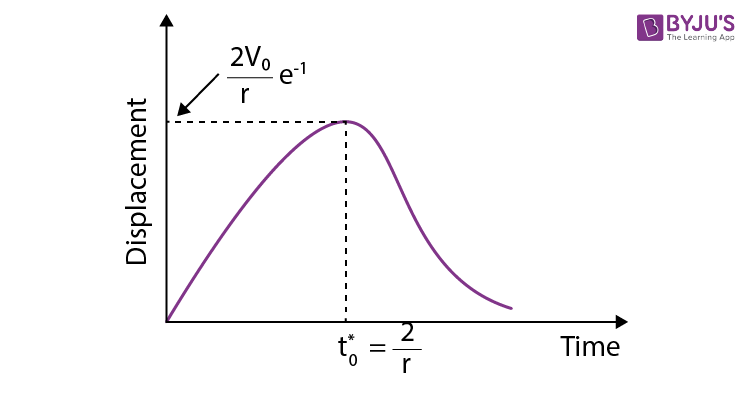
Figure 2 is a graph of x against t in Equation (3.13). It illustrates the displacement – time behaviour of a damped system with
\(\begin{array}{l}\gamma =2{{\omega }_{0}},\end{array} \)
when it is disturbed from equilibrium by a sudden impulse For small values of t, the term \(\begin{array}{l}{{e}^{-\gamma t/2}}\end{array} \)
is very nearly unity and displacement [Equation (3.13)], which increase linearly with time t. After some time, \(\begin{array}{l}{{e}^{-\gamma t/2}}\end{array} \)
starts changing, and the displacement decays exponentially with time, eventually becoming zero. The turning point occurs at a time t0, when \(\begin{array}{l}\frac{dx}{dt}=0.\end{array} \)
From Eq. (3.14), this happens at t = t0 given by
\(\begin{array}{l}1-\frac{\gamma {{t}_{0}}}{2}=0\end{array} \)
Or
\(\begin{array}{l}{{t}_{0}}=\frac{2}{\gamma }=\frac{1}{{{\omega }_{0}}}\end{array} \)
The displacement increases until time t = t0, after which it decays to zero. A comparison of Equations (3.8) and (3.13) reveals that the decay rate is much faster when γ = 2ω0 than when γ > 2ω0. In both cases, there is no oscillation at all since ψ never becomes negative.
The motion described by Equation (3.13) is called critically damped. The necessary condition for critical damping is γ = 2ω0. Suppose we are faced with a problem in which we desire a high rate of decay without oscillation. Evidently, the optimum choice is critical damping. We come across such a problem in pointer-type galvanometers, where we would want the pointer to move immediately to the correct position and stay there without annoying oscillation (see sec. 3.6).
Case III \(\begin{array}{l}\gamma <2\,{{\omega }_{0}}\end{array} \)
(Small Damping).
When γ < 2ω0, the damping is small, and this gives the most important kind of behaviour, namely, oscillatory damped harmonic motion, for then, the expression
\(\begin{array}{l}{{\left( \frac{{{\gamma }^{2}}}{4}-\omega _{0}^{2} \right)}^{1/2}}\end{array} \)
in the exponentials in Eq. (3.5) is an imaginary quantity. Writing this as
\(\begin{array}{l}{{\left( \frac{{{\gamma }^{2}}}{4}-\omega _{^{0}}^{2} \right)}^{1/2}}=\sqrt{-1}\left( \omega _{0}^{2}-\frac{{{\gamma }^{2}}}{4} \right)^{1/2}\end{array} \)
\(\begin{array}{l}=i\omega *\end{array} \)
Where,
\(\begin{array}{l}\omega *={{\left( \omega _{0}^{2}-\frac{{{\gamma }^{2}}}{4} \right)}^{1/2}}\end{array} \)
is a real positive quantity, the displacement Equation (3.5) may be rewritten as
\(\begin{array}{l}x={{e}^{-\gamma t/2}}\left\{ \left( {{A}_{1}}\exp \left( i\omega *t \right)+{{A}_{2}}\exp \left( -i\omega *t \right) \right) \right\}….(3.15)\end{array} \)
To compare the behaviour of a damped oscillator with the ideal case in which damping is ignored, we will recast Equation (3.15) into a more familiar form. We can do this by using the identities,
\(\begin{array}{l}{{e}^{i\theta }}=\cos \theta +i\sin \theta\end{array} \)
\(\begin{array}{l}{{e}^{-i\theta }}=\cos \theta -i\sin \theta\end{array} \)
So that Equation (3.15) can be written as
\(\begin{array}{l}x={{e}^{-\gamma t/2}}\left\{ \left( {{A}_{1}}+{{A}_{2}} \right)\cos \omega *t+i\left( {{A}_{1}}-{{A}_{2}} \right)\sin \omega *t \right\}\end{array} \)
If we choose
\(\begin{array}{l}{{A}_{1}}+{{A}_{2}}=A\cos \delta\end{array} \)
\(\begin{array}{l}i\left( {{A}_{1}}-{{A}_{2}} \right)=A\sin \delta\end{array} \)
Where A and δ are constants which depend upon the initial conditions, we find, after the substitution,
\(\begin{array}{l}x=A\,{{e}^{-\gamma t/2}}\cos \left( \omega *t-\delta \right)….(3.16)\end{array} \)
With
\(\begin{array}{l}\omega *={{\omega }_{0}}{{\left( 1-\frac{{{\gamma }^{2}}}{4\omega _{0}^{2}} \right)}^{1/2}}….(3.17)\end{array} \)
Differentiating Eq. (3.16), we obtain an expression for the velocity of the oscillator, which reads
\(\begin{array}{l}\frac{dx}{dt}=-A\,\,{{e}^{-\gamma t/2}}\left\{ \omega *\sin \left( \omega *t-\delta \right)+\frac{\gamma }{2}\cos \left( \omega *t-\delta \right) \right\}….(3.18)\end{array} \)
Equation (3.16) shows that the motion is oscillatory. The oscillation is not simple harmonic since its ‘amplitude’
\(\begin{array}{l}A\,{{e}^{-\gamma t/2}}\end{array} \)
is not constant but decreases with time. The motion is not periodic since it never repeats itself, each swing being of smaller amplitude than the preceding one. However, if γ is very small compared to ω0, the amplitude will remain sensibly constant over a large number of cycles of the harmonic term \(\begin{array}{l}\cos \left( \omega *t-\delta \right)\end{array} \)
, in that case, the motion is nearly periodic and simple harmonic.
The angular frequency of the oscillation is ω* given Equation (3.17), which is less than the natural angular frequency of free undamped oscillations. Strictly speaking, we are really not justified in using the terms ‘amplitude’ and ‘frequency’ for a motion which is not periodic. But, when damping is small, the motion is nearly periodic; we may use these terms with some reservations.
To illustrate the behaviour of a weakly damped oscillator, let us choose the initial conditions, namely, that at t = 0, x = 0 and
\(\begin{array}{l}\frac{dx}{dt}={{V}_{0}}.\end{array} \)
. Using these conditions in Equations (3.16) and (3.18), we get
\(\begin{array}{l}0=A\cos \delta\end{array} \)
And
\(\begin{array}{l}{{V}_{0}}=-A\left( \frac{\gamma }{2}\cos \delta -\omega *\sin \delta \right)\end{array} \)
yielding
\(\begin{array}{l}\delta =\frac{\pi }{2}\end{array} \)
(A = 0; being a trivial case)
And
\(\begin{array}{l}A=\frac{{{V}_{0}}}{\omega *}\end{array} \)
Using these values of A and δ in Equations (3.16) and (3.18), we find that, under the above initial conditions, the displacement and velocity of the oscillator are, respectively, given by
\(\begin{array}{l}x=\frac{{{V}_{0}}}{\omega *}{{e}^{-\gamma t/2}}\sin \omega *t=A\left( t \right)\sin \omega *t\end{array} \)
With
\(\begin{array}{l}A\left( t \right)=\frac{{{V}_{0}}}{\omega *}{{e}^{-\gamma t/2}}={{A}_{0}}{{e}^{-\gamma t/2}}\end{array} \)
A0 being the value of A(t) when γ = 0
And
\(\begin{array}{l}\frac{dx}{dt}={{V}_{0}}\,{{e}^{-\gamma t/2}}\left( \cos \omega *t-\frac{\gamma }{2\omega *}\sin \omega *t \right)….(3.20)\end{array} \)
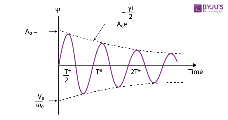
Figure 3.4 depicts the behaviour of a weakly damped oscillator. It is a graph of ψ against t of the motion described by Equation (3.19). The constant A0 is the value of
\(\begin{array}{l}A\left( t \right)=\frac{{{V}_{0}}}{\omega *}{{e}^{-\gamma t/2}}\end{array} \)
in the absence of damping (γ = 0), i.e. \(\begin{array}{l}{{A}_{0}}={{V}_{0}}/\omega *.\end{array} \)
. Since the maximum values of \(\begin{array}{l}\sin \left( \omega *t \right)\end{array} \)
are + 1 and -1 alternately, the displacement-time graph of oscillation is bounded by the dotted curves \(\begin{array}{l}{{A}_{0}}{{e}^{-\gamma t/2}}\end{array} \)
and \(\begin{array}{l}-{{A}_{0}}{{e}^{-\gamma t/2}}\end{array} \)
.
Thus, although the amplitude decreases exponentially with time, the weekly damped oscillator executes some sort of oscillatory motion. The motion does not repeat itself and is, therefore, not periodic in the usual sense of the term. However, it still has a time period
\(\begin{array}{l}T*=2\pi /\omega *,\end{array} \)
, which is the time interval between two alternate zeros of displacement. The time period between two successive zeros of displacement is T*/2. This is also the time interval between a maximum and minimum value of the displacement, but the maxima and minima are not exactly halfway between the zeros. This is obvious from Equation (3.20) because, at a maximum or a minimum displacement, the velocity is zero, giving
\(\begin{array}{l}\cos \omega *t-\frac{\gamma }{2\omega *}\sin \omega *t=0\end{array} \)
Or
\(\begin{array}{l}\tan \omega *t=\frac{2\omega *}{\gamma }\end{array} \)
Displacement-time behaviour of a weakly damped oscillator,
The values of t satisfying this equation are the instants at which ψ is either a positive maximum or a negative maximum. In the case when
\(\begin{array}{l}\gamma <2{{\omega }_{0}},\frac{2{{\omega }_{0}}}{\gamma }\to \infty ,\end{array} \)
so that
\(\begin{array}{l}\omega *t\to \frac{\pi }{2},\frac{3\pi }{2},\frac{5\pi }{2},…,\end{array} \)
The first maximum of ψ occurs at a time
\(\begin{array}{l}t={{t}_{1}}\end{array} \)
given by
\(\begin{array}{l}\omega *{{t}_{1}}=\frac{\pi }{2}\end{array} \)
Or
\(\begin{array}{l}{{t}_{1}}=\frac{\pi }{2\omega *}=\frac{T*}{4}\end{array} \)
i.e., the maximum is exactly midway between the two zeros of ψ. Thus, only in the case of negligibly small damping are the maxima and minima halfway between the zeros of displacement as in the case of simple harmonic motion.
Effect of Damping:
The effect of damping is two-fold: (a) The amplitude of oscillation decreases exponentially with time as
\(\begin{array}{l}A\left( t \right)={{A}_{0}}{{e}^{-\gamma t/2}}\end{array} \)
Where, A0 is the amplitude in the absence of damping and (b) The angular frequency ω* of the damped oscillator is less than ω0, the frequency of the undamped oscillation. The relation between them is
\(\begin{array}{l}\omega *={{\omega }_{0}}{{\left( 1-\frac{{{\gamma }^{2}}}{4\omega _{0}^{2}} \right)}^{1/2}}\end{array} \)
Energy of a Weakly Damped Oscillator
We shall now develop an expression for the average energy of a weakly damped oscillator at any instant of time. We have seen that, in the case of weak damping
\(\begin{array}{l}\left( \gamma <2{{\omega }_{0}} \right),\end{array} \)
, the displacement and velocity of the oscillator are, respectively given by Equations (3.16) and (3.18). If m is the mass of the oscillator, its instantaneous kinetic energy is
\(\begin{array}{l}\frac{1}{2}m{{\left( \frac{dx}{dt} \right)}^{2}}\end{array} \)
Which, with the help of Equation (3.18), becomes
\(\begin{array}{l}KE =\frac{1}{2}m{{A}^{2}}{{e}^{-\gamma t}}{{\left\{ \omega *\sin \left( \omega *t-\delta \right)+\frac{\gamma }{2}\cos \left( \omega *t-\delta \right) \right\}}^{2}}\end{array} \)
\(\begin{array}{l}=\frac{1}{2}m{{A}^{2}}{{e}^{-\gamma t}}\left\{ \omega {{*}^{2}}{{\sin }^{2}}\left( \omega *t-\delta \right)+\omega *\gamma \sin \left( \omega *t-\delta \right)\cos \left( \omega *t-\delta \right)+\frac{{{\gamma }^{2}}}{4}{{\cos }^{2}}\left( \omega *t-\delta \right) \right\}\end{array} \)
The instantaneous potential energy of the oscillator is given by
\(\begin{array}{l}PE=\int\limits_{0}^{x}{Kx}dx=\frac{1}{2}K{{x}^{2}}\end{array} \)
Using Equation (3.16), we have
\(\begin{array}{l}K=m\omega _{0}^{2},\end{array} \)
\(\begin{array}{l}PE=\frac{1}{2}m\omega _{0}^{2}{{A}^{2}}{{e}^{-\gamma t}}{{\cos }^{2}}\left( \omega *t-\delta \right)\end{array} \)
The total energy of the oscillator at any instant of time is then given by
\(\begin{array}{l}E\left( t \right)=KE+PE\end{array} \)
\(\begin{array}{l}=\frac{1}{2}m\,{{A}^{2}}{{e}^{-\gamma t}}\left\{ \omega {{*}^{2}}{{\sin }^{2}}\left( \omega *t-\delta \right)+\frac{\omega *\gamma }{2}\sin 2\left( \omega *t-\delta \right)+\left( \frac{{{\gamma }^{2}}}{4}+\omega _{0}^{2} \right){{\cos }^{2}}\left( \omega *t-\delta \right) \right\}\end{array} \)
….(3.21)
If damping is very small
\(\begin{array}{l}\left( \gamma <2{{\omega }_{0}} \right),\end{array} \)
as is usually the case, the term \(\begin{array}{l}{{e}^{-\gamma t}}\end{array} \)
in Eq. (3.21) does not change appreciably during one time period \(\begin{array}{l}T*=2\pi /\omega *\end{array} \)
of the oscillation. Thus, assuming that \(\begin{array}{l}{{e}^{-\gamma t}}\end{array} \)
is sensibly constant during period T* of the oscillations, the time-averaged energy of the oscillator is given by
\(\begin{array}{l}<E\left( t \right)>=\frac{1}{2}m{{A}^{2}}\,{{e}^{-\gamma t}}\left\{ \omega {{*}^{2}}<{{\sin }^{2}}\left( \omega *t-\delta \right)>+\frac{\omega *\gamma }{2}<\sin 2\left( \omega *t-\delta \right)>+\left( \frac{{{\gamma }^{2}}}{4}+\omega _{0}^{2} \right)<{{\cos }^{2}}\left( \omega *t-\delta \right)> \right\}\end{array} \)
……(3.22)
Where notation < > implies averaging over a one-time period T*. A function f(t) averaged over T is, by definition, given by
\(\begin{array}{l}<f\left( t \right)>=\frac{\int\limits_{0}^{T}{f\left( t \right)dt}}{\int\limits_{0}^{T}{dt}}=\frac{1}{T}\int\limits_{0}^{T}{f\left( t \right)dt}\end{array} \)
Thus,
\(\begin{array}{l}<{{\sin }^{2}}\left( \omega *t-\delta \right)>=\frac{1}{T*}\int\limits_{0}^{T*}{{{\sin }^{2}}}{{\left( \frac{2\pi t}{T*}-\delta \right)}^{2}}dt\end{array} \)
To integrate, let us use the transformation
\(\begin{array}{l}\frac{2\pi t}{T*}-\delta =\alpha\end{array} \)
So that
\(\begin{array}{l}dt=\frac{T*}{2\pi }d\infty\end{array} \)
Then,
\(\begin{array}{l}<{{\sin }^{2}}\left( \omega *t-\delta \right)>=\frac{1}{2\pi }\int\limits_{-\delta }^{2\pi -\delta }{{{\sin }^{2}}\alpha dx}=\frac{1}{4\pi }\int\limits_{0}^{2\pi }{\left( 1-\cos 2\alpha \right)dx=\frac{1}{2}}\end{array} \)
Similarly,
\(\begin{array}{l}<{{\cos }^{2}}\left( \omega *t-\delta \right)>=\frac{1}{2}\end{array} \)
And
\(\begin{array}{l}<\sin 2\left( \omega *t-\delta \right)>=0\end{array} \)
Substituting for these time-averaged values in Equation (3.22), we get
\(\begin{array}{l}<E\left( t \right)>=\frac{1}{4}m{{A}^{2}}{{e}^{-\gamma t}}\left( \omega {{*}^{2}}+\frac{{{\gamma }^{2}}}{4}+\omega _{0}^{2} \right)\end{array} \)
Now, since
\(\begin{array}{l}\omega {{*}^{2}}=\omega _{0}^{2}-\frac{{{\gamma }^{2}}}{4},\end{array} \)
we have
\(\begin{array}{l}<E\left( t \right)>=\frac{1}{2}m{{A}^{2}}\omega _{0}^{2}{{e}^{-\gamma t}}\end{array} \)
Or
\(\begin{array}{l}<E\left( t \right)>={{E}_{0}}{{e}^{-\gamma t}}\end{array} \)
Where
\(\begin{array}{l}{{E}_{0}}=\frac{1}{2}m{{A}^{2}}\omega _{0}^{2},\end{array} \)
is the total energy of an undamped oscillator. Hence, the energy of a weakly damped oscillator diminishes exponentially with time. The decay of the total energy is illustrated in the figure below.
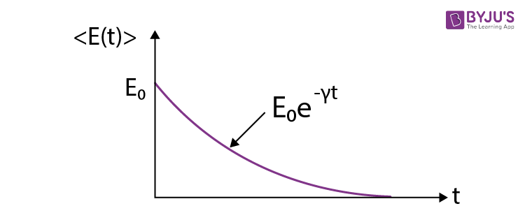
Figure: Exponential decay of total energy during damping of harmonic oscillations
The average power dissipation during one time period is given by
< P (t) > = rate of loss of energy
\(\begin{array}{l}=\frac{d}{dt}<E\left( t \right)>\end{array} \)
\(\begin{array}{l}=\gamma {{E}_{0}}\,{{e}^{-\gamma t}}\end{array} \)
\(\begin{array}{l}=\gamma <E\left( t \right)>\end{array} \)
This expression may also be obtained as follows: Since the loss of energy is due to work done by the oscillator to overcome the force of friction
\(\begin{array}{l}F=-p\frac{dx}{dt},\end{array} \)
the instantaneous power P(t) is given by
\(\begin{array}{l}P\left( t \right)=\frac{\text{work}}{\text{time}}=\frac{F.\delta x}{\delta t}=F\frac{dx}{dt}\end{array} \)
Where δψ is the change in displacement in time δt. Thus
\(\begin{array}{l}P\left( t \right)=p{{\left( \frac{dx}{dt} \right)}^{2}}=m\gamma {{\left( \frac{dx}{dt} \right)}^{2}}\end{array} \)
….(3.24)
Now using Equation (3.18), we have,
\(\begin{array}{l}P\left( t \right)=m\gamma {{A}^{2}}{{e}^{-\gamma t}}\left\{ \omega {{*}^{2}}{{\sin }^{2}}\left( \omega *t-\delta \right)+\frac{\omega *\gamma }{2}\sin 2\left( \omega *t-\delta \right)+\frac{{{\gamma }^{2}}}{4}{{\cos }^{2}}\left( \omega *t-\delta \right) \right\}\end{array} \)
Hence, the power dissipation during one time period of oscillation is given by
\(\begin{array}{l}<P\left( t \right)>=m\gamma {{A}^{2}}{{e}^{-\gamma t}}\left\{ \omega {{*}^{2}}<{{\sin }^{2}}\left( \omega *t-\delta \right)>+\frac{\omega *\gamma }{2}<\sin 2\left( \omega *t-\delta \right)>+\frac{{{\gamma }^{2}}}{4}<{{\cos }^{2}}\left( \omega *t-\delta \right)> \right\}\end{array} \)
\(\begin{array}{l}=\frac{1}{2}\gamma \,m\,{{A}^{2}}\,{{e}^{-\gamma t}}\left( \omega {{*}^{2}}+\frac{{{\gamma }^{2}}}{4} \right)\end{array} \)
\(\begin{array}{l}=\frac{1}{2}\,\gamma m{{A}^{2}}\omega _{0}^{2}{{e}^{-\gamma t}}\end{array} \)
\(\begin{array}{l}=\gamma <E\left( t \right)>\end{array} \)
…..(3.25)
As mentioned earlier, this loss of energy is due to friction in the system (leading to heating) and the emission of radiation from the system (resulting in waves).
Frequently Asked Questions on Damped Oscillation
Q1
What is damped oscillation?
Damped oscillations are periodic oscillations whose amplitude decreases gradually with time.
Q2
What is an undamped oscillation?
The periodic oscillations whose amplitude decreases with the passage of time are called undamped oscillations.
Q3
Give two examples of damped oscillations.
Oscillations of the bob of a simple pendulum in the laboratory.
Oscillations of a swing in the air.

Comments