The intercept in linear regression represents:

the expected y value when x is zero

the strength of the relationship between x and y

the expected x value when y is zero

Statistics - Study Material for IIT JEE & Solved Examples

The word statistics is derived from the Latin word “status” which means a state. Statistics normally means taking the values of some parameters and by plotting it or by arranging it in a meaningful manner. Basically, statistics give us the process by which we can collect, analyze, interpret, present and organize data.

In statistics, we normally use words like “mean”, ”median” and “mode” to understand the data distributed throughout a range. Be it grouped or ungrouped, usually, these central tendency measures give a single data point which typically shows the behaviour of the whole data.

Also, Check:

Previous Years IIT JEE Questions on Statistics

Types of Averages

By averages, we normally mean the mean, median and mode of any data set.

MEAN

Mean is the simple average of a data set, i.e., mean can be represented by:

\(\begin{array}{l}\bar{x}=\frac{(sum of the observations)}{(count of the observations)}\end{array} \)

In the mathematical sense, mean is called average, but the two words don’t mean the same, all the time.

Let us take an example:

(In the case of discrete data)

The marks obtained by 10 students in a class are 56, 54, 89, 74, 23, 16, 94, 52, 68, 100.

So, the mean of the data presented will be given by:

\(\begin{array}{l}\bar{x}=\frac{(56+54+89+74+23+16+94+52+68+100)}{10}\end{array} \)

= 626/10

= 62.6

Now, let us take the case of grouped data.

The table shows the marks obtained by 10 students will be:

Marks	No. of students	Mid-point(x)	Value(x)
0-10	1	5	5
11-20	5	15.5	77.5
21-30	2	25.5	51
31-40	3	35.5	106.5
41-50	6	45.5	273
51-60	8	55.5	444
61-70	1	65.5	65.5
71-80	5	75.5	377.5
81-90	4	85.5	342
91-100	2	95.5	191

1st Step: We have to find the mid-points of every class and the interval is 10.

2nd Step: It will be the multiplication of the midpoint by the class frequency.

3rd Step: Then we sum the frequency and divide it by the frequency to get the mean.

\(\begin{array}{l}\bar{x}=\frac{(5+77.5+51+106.5+273+444+65.5+377.5+342+191)}{10}\end{array} \)

= 1933/10

= 193.3

MEDIAN

Median basically means the middle-most value in a data set. In case of an ungrouped data, firstly we will arrange the entire data set in ascending order. Now, if the number of terms is odd, we find the median by finding out the value of ((n+1)/2)th term and if the number of terms is even, the median will be given by the average of (n/2)th term and ((n+1)/2)th term

Median calculation for grouped data:

Step 1: Find the class mark x_i for each class.

Step 2: Find N = ∑ f_i

Step 3: Take the median class to be that value whose cumulative frequency is near about (N/2)

Step 4: Calculate the median by the following value:

\(\begin{array}{l}M = l+\frac{\frac{N}{2}-c}{f}\times h\end{array} \)

l = lower limit of the median class

f = frequency of the median class

h = width of the median class

c = cumulative frequency of the class just preceding the median class

MODE

By mode, we usually represent the maximum occurrence of a single element in a series of elements. This also represents a measure of central tendency. Sometimes, a series has only elements with an occurrence of one time only, some have zero occurrences, and some have more than one.

Video Lesson: Mean, Median and Mode

Dispersion in Statistics

By dispersion, we normally mean the extent to which the data is distributed or spread. It usually gives us a measure of the variation of every single data point from the average of all the points in a data set.

Now we can calculate dispersion by two types:

Absolute value of the dispersion
Relative value of the dispersion

Absolute Value of Dispersion

This takes into account the expression of the data with respect to the original data. They cannot be used to compare two or more data sets and tell us whether the data is highly scattered or not.

This includes:

Range
Mean Deviation
Variance
Standard Deviation

Range:

We normally find the range by subtracting the minimum value from the maximum value in a data set. We cannot tell how much the data are dispersed or scattered- so, it is better that we introduce standard, mean and quartile deviation.

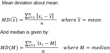
Mean Deviation:

The mean deviation tells us about the deviation from the mean or median data.

The formula of mean deviation is given by:

Mean Deviation Formula in Statistics

Variance

Sometimes we have to take the mean deviation by taking the absolute values from a set of values. The absolute values were taken to measure the deviations, as otherwise, the positive and negative deviation may cancel out each other.

So, to remove the sign of deviation, we usually take the variance of the data set, i.e., we usually square the deviation values. As squares are always positive, so the variance is always a positive number.

Let us take “n” observations as a₁, a₂, a₃, ….., a_n

\(\begin{array}{l}\text{and their mean is represented by}\ \bar{a}.\end{array} \)

Then the variance is denoted by

\(\begin{array}{l}\sigma^2 = (a_1- \bar a)^2 +(a_2- \bar a)^2+(a_3- \bar a)^2 + …..+(a_n – \bar a)^2 = \sum_{i=1}^n (a_i- \bar{a})^2\end{array} \)

Properties of Variance

If the variance comes out to be zero, this means that
\(\begin{array}{l}(a_i – \bar{a})\ \text{is equal to zero, }\end{array} \)

\(\begin{array}{l}\text{which is nothing but each value of the set is equal to the mean value}\ \bar{a}.\end{array} \)
If the variance is small,
\(\begin{array}{l}\text{it means that the observations are pretty close to the mean value}\ \bar{a}.\end{array} \)
If the value is greater,
\(\begin{array}{l}\text{the deviations of the observations are far from the mean value}\ \bar{a}.\end{array} \)
If each observation is increased by a where a ∈ R, then the variance will remain unchanged.
If each observation is multiplied by a where a ∈ R, then the variance will be multiplied by a² also.
But for some data sets, the variance by the formula
\(\begin{array}{l}\sum_{i=1}^n (a_i – \bar{a})^2\end{array} \)
does not give the proper values as the range of deviation may vary, and the observations may be more scattered about the mean. So, to overcome this difficulty, we take the mean of the square of the deviations.

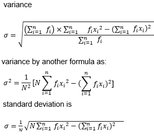
So, the variance is given by:

\(\begin{array}{l}\sigma^2 = \frac{1}{n} \sum_{i=1}^n (a_i – \bar a)^2\end{array} \)

As a result of squaring, the unit of variance is not the same as that of the data sets taken.

Standard Deviation

To take a proper measure of dispersion, we have to calculate the standard deviation by taking the square root of the variance. This measure often prevents above-average deviations from cancelling those below, which can sometimes contribute to a null variance. If the variance is great, then the standard deviation will be more, and for lesser variance, the opposite case occurs.

The formula of standard deviation is given by:

\(\begin{array}{l}\sigma = \sqrt{\sigma^2} = \sqrt{\frac{1}{n} \sum_{i=1}^n (a_i – \bar a)^2}\end{array} \)

Standard Deviation of distribution with discrete frequency:

It is given by:

\(\begin{array}{l}\sigma = \sqrt{\frac{1}{n} \sum_{i=1}^n (f_i a_i – \bar a)^2}\end{array} \)

Where the values are: a₁, a₂, a₃,…., a_n

And the respective frequencies are: f₁, f₂, f₃,…., f_n

And

\(\begin{array}{l}N = \sum_{i=1}^n f_i\end{array} \)

Standard Deviation of distribution with continuous frequency:

Relative Value of Dispersion

By this method, we represent the scattering in terms of some values, i.e., either in percentage or in the form of a ratio. This is mainly helpful to compare three or more data sets simultaneously.

The different forms of the relative measures of dispersion are:

● Coefficient of Range

● Coefficient of Mean Deviation

● Coefficient of Variance and Standard Deviation

Coefficient of Range

It is defined as the ratio of the difference between the highest and lowest values to the sum of the two.

It is given by;

\(\begin{array}{l}\frac{x_m-x_o}{x_m+x_o }\end{array} \)

Coefficient of Mean Deviation

It is defined as the ratio of the mean deviation to the mean of the same data set.

It is given by (Mean deviation from Mean)/Mean or (Mean deviation from Median)/Median

Solved Examples

Example 1: An experiment is conducted with 16 values of b, and the following results were obtained. ∑ b² = 2560 and ∑ b = 180. On checking through the data again, it is seen that one observation with a particular value 30 is replaced with 20. What will be the corrected variance?

Solution:

Given: ∑ b² = 2560 and ∑ b = 180

So, ∑ b¹ = 180 – 30 + 20 = 170

And the variance will be decreased by ∑ b² = 900 – 400 = 500

The value of variance becomes ∑ b² = 2560 – 900 + 400 = 2060

So, the corrected variance = 1/n ∑ (b² -[1/n ∑ b¹]² )

= (1/16) × 2060 – (1/16 × 170)²

= 128.75 – 112.890625

= 15.859375

Example 2: Calculate the median for the following data:

Marks	0-10	10-20	20-30	30-40	40-50
No. of Students	5	15	20	2	8

Solution: First, we will calculate the cumulative frequency and mid-point.

Marks	Frequency	Cumulative frequency	Mid-point
0-10	5	5	5
10-20	15	20	15
20-30	20	40	25
30-40	2	42	35
40-50	8	50	45

Thus, N = 50 and N/2 = 25

So, the median class is 20-30.

l = 20, f = 20, h = 10 and c = 20

So, median = 20 + [(25 – 20)/20] × 10 = 22.5

Example 3:

Let us take two sets of values where one set is represented by the scores of 100 Indian batsmen, and the other represents the scores of 100 Australian batsmen. Incidentally, the Indians have scored runs in the order 550, 551, 552, ….., 649. And the Australian batsmen have scored runs in the order 900, 901, 902, …., 999. If the variances of the two sets are represented by σ_A and σ_B, then what will be the value of σ_A /σ_B?

Solution:

We know,

\(\begin{array}{l}\sigma^2 = \frac{\sum d_i^2}{n}\end{array} \)

Here, both the Australian and Indian batsmen have 100 consecutive positive integers and the value of n = 100, which is also the same.

\(\begin{array}{l}\text{Thus},\ \sum d_i^2\ \text{is the same for both of these integer sets.}\end{array} \)

So, σ_A /σ_B =1

Example 4: The S.D. of a variate x is s. The S.D. of the variate (ax + b)/c, where a, b, c are constant, is

\(\begin{array}{l}A) \left( \frac{a}{c} \right)\,\sigma\\ B) \left| \frac{a}{c} \right|\,\sigma\\ C) \left( \frac{{{a}^{2}}}{{{c}^{2}}} \right)\,\sigma \\ D)\ \text{None of these}\end{array} \)

Solution:

Let

\(\begin{array}{l}y=\frac{ax+b}{c}\\ y=\frac{a}{c}x+\frac{b}{c}\\ y=Ax+B,\end{array} \)

where

\(\begin{array}{l}A=\frac{a}{c},B=\frac{b}{c} \\ \bar{y}=A\bar{x}+B\\ y-\bar{y}=A(x-\bar{x})\\ {{(y-\bar{y})}^{2}}={{A}^{2}}{{(x-\bar{x})}^{2}}\\ \sum {{(y-\bar{y})}^{2}}={{A}^{2}}\sum {{(x-\bar{x})}^{2}}\\ n.\sigma _{y}^{2}={{A}^{2}}.n\sigma _{x}^{2}\\ \sigma _{y}^{2}={{A}^{2}}\sigma _{x}^{2}\\ {{\sigma }_{y}}=\,|A|{{\sigma }_{x}}\\ {{\sigma }_{y}}=\,\left| \frac{a}{c} \right|{{\sigma }_{x}}\end{array} \)

Example 5: Let r be the range and

\(\begin{array}{l}{{S}^{2}}=\frac{1}{n-1}\sum\limits_{i=1}^{n}{{{({{x}_{i}}-\bar{x})}^{2}}}\end{array} \)

be the S.D. of a set of observations x₁, x₂, …., x_n, then

\(\begin{array}{l}A) S\le r\sqrt{\frac{n}{n-1}}\\ B) S=r\sqrt{\frac{n}{n-1}}\\ C) S\ge r\sqrt{\frac{n}{n-1}}\\ D)\ \text{None of these}\end{array} \)

Solution:

We have

\(\begin{array}{l}\underset{\,\,\,\,\,\,\,\,\,\,\,\,\,i\,\ne j}{\mathop{r=\max |{{x}_{i}}-{{x}_{j}}|}}\,\end{array} \)

and

\(\begin{array}{l}{{S}^{2}}=\frac{1}{n-1}\sum\limits_{i=1}^{n}{{{({{x}_{i}}-\bar{x})}^{2}}}\end{array} \)

Now

\(\begin{array}{l}{{({{x}_{i}}-\bar{x})}^{2}}={{\left( {{x}_{i}}-\frac{{{x}_{1}}+{{x}_{2}}+…..+{{x}_{n}}}{n} \right)}^{2}}\\ =\frac{1}{{{n}^{2}}}[({{x}_{i}}-{{x}_{1}})+({{x}_{i}}-{{x}_{2}})+….+({{x}_{i}}-{{x}_{i}}-1)\\ +({{x}_{i}}-{{x}_{i}}+1)+…….+({{x}_{i}}-{{x}_{n}})]\le \frac{1}{{{n}^{2}}}{{[(n-1)r]}^{2}},[\because |{{x}_{i}}-{{x}_{j}}|\le r]\\ {{({{x}_{i}}-\bar{x})}^{2}}\le {{r}^{2}}\Rightarrow \sum\limits_{i=1}^{n}{{{({{x}_{i}}-\bar{x})}^{2}}\le n{{r}^{2}}}\\ \frac{1}{n-1}\sum\limits_{i=1}^{n}{{{({{x}_{i}}-\bar{x})}^{2}}\le \frac{n{{r}^{2}}}{(n-1)}}\\ {{S}^{2}}\le \frac{n{{r}^{2}}}{(n-1)}\\ S\le r\sqrt{\frac{n}{n-1}}.\end{array} \)

Example 6: The mean and S.D. of the marks of 200 candidates were found to be 40 and 15, respectively. Later, it was discovered that a score of 40 was wrongly read as 50. The correct mean and S.D., respectively, are

A) 14.98, 39.95

B) 39.95, 14.98

C) 39.95, 224.5

D) None of these

Solution:

\(\begin{array}{l}\text{Corrected}\ \Sigma x=40\times 200-50+40=7990\end{array} \)

\(\begin{array}{l}\text{Corrected}\ \bar{x}=7990/200=39.95\end{array} \)

\(\begin{array}{l}\text{Incorrect}\ \Sigma {{x}^{2}}=n\,[{{\sigma }^{2}}+{{\bar{x}}^{2}}]=200[{{15}^{2}}+{{40}^{2}}]=365000\end{array} \)

\(\begin{array}{l}\text{Correct}\ \Sigma {{x}^{2}}=365000-2500+1600=364100\end{array} \)

\(\begin{array}{l}\text{Corrected}\ \sigma = \sqrt{\frac{364100}{200}-{{(39.95)}^{2}}}\\=\sqrt{(1820.5-1596)}\\=\sqrt{224.5}\\=14.98.\end{array} \)

Example 7: The average of n numbers x₁, x₂, x₃, …., x_n is M. If x_n is replaced by x’, then the new average is

\(\begin{array}{l}A) M-{{x}_{n}}+{x}’\\ B) \frac{nM-{{x}_{n}}+{x}’}{n}\\ C) \frac{(n-1)M+{x}’}{n}\\ D) \frac{M-{{x}_{n}}+{x}’}{n}\end{array} \)

Solution:

\(\begin{array}{l}M=\frac{{{x}_{1}}+{{x}_{2}}+{{x}_{3}}……{{x}_{n}}}{n}\\ \underset{n}{\mathop{\underline{\begin{matrix} nM \\ nM-{{x}_{n}} \\ nM-{{x}_{n}}+{x}’ \\ \end{matrix}}}}\,\begin{matrix} = \\ = \\ = \\ \end{matrix}\underset{n}{\mathop{\underline{\begin{matrix} {{x}_{1}}+{{x}_{2}}+{{x}_{3}}+……{{x}_{n-1}}+{{x}_{n}} \\ {{x}_{1}}+{{x}_{2}}+{{x}_{3}}+……{{x}_{n-1}}\ \ \ \ \ \\ {{x}_{1}}+{{x}_{2}}+{{x}_{3}}+……{{x}_{n-1}}+{x}’ \\ \end{matrix}}}}\,\end{array} \)

Hence, the new average

\(\begin{array}{l}=\frac{nM-{{x}_{n}}+{x}’}{n}\end{array} \)

Statistics for IIT JEE

Types of Averages

MEAN

MEDIAN

MODE

Video Lesson: Mean, Median and Mode

Dispersion in Statistics

Absolute Value of Dispersion

Relative Value of Dispersion

Solved Examples

Statistics – Important Topics

Statistics for IIT JEE in One-Shot

Comments

Leave a Comment Cancel reply

FREE TEXTBOOK SOLUTIONS